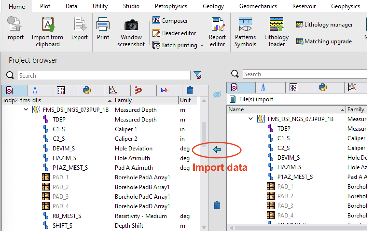
Loading processed FMS images from logDB into TechLog
The data in the LogDB processed DLIS files have all been corrected
for tool motion and depth matched to other data, but the various
arrays need to be recombined in order to be able to display and
interpret the images. The procedure depends on the software used for
the original processing (GeoFrame until 2017; TechLog after):
For data processed with GeoFrame (All ODP data, and IODP data through IODP Expedition 367): individual 'buttons' need to be combined into into image arrays, which are then used to create Pad images, that are finally
concatenated into oriented images.
For data processed with TechLog (from IODP Expedition 369 onwards) (as well as IODP Hole 311-U1328C):
the Pad images are already part of the processed dlis file and the data
only need to be loaded before being oriented.
For all data, the recommended final step is the equalization, or
normalization, of the images, which typically enhances the images
and makes the interpretation easier.
The first version of this document was started with an earlier
version of Techlog, and it was later upgraded with newer versions. Some
appearances may be different from the current versions, but the
procedure is the same.
Data processed with GeoFrame (until IODP Expedition 367)
Importing the DLIS file:
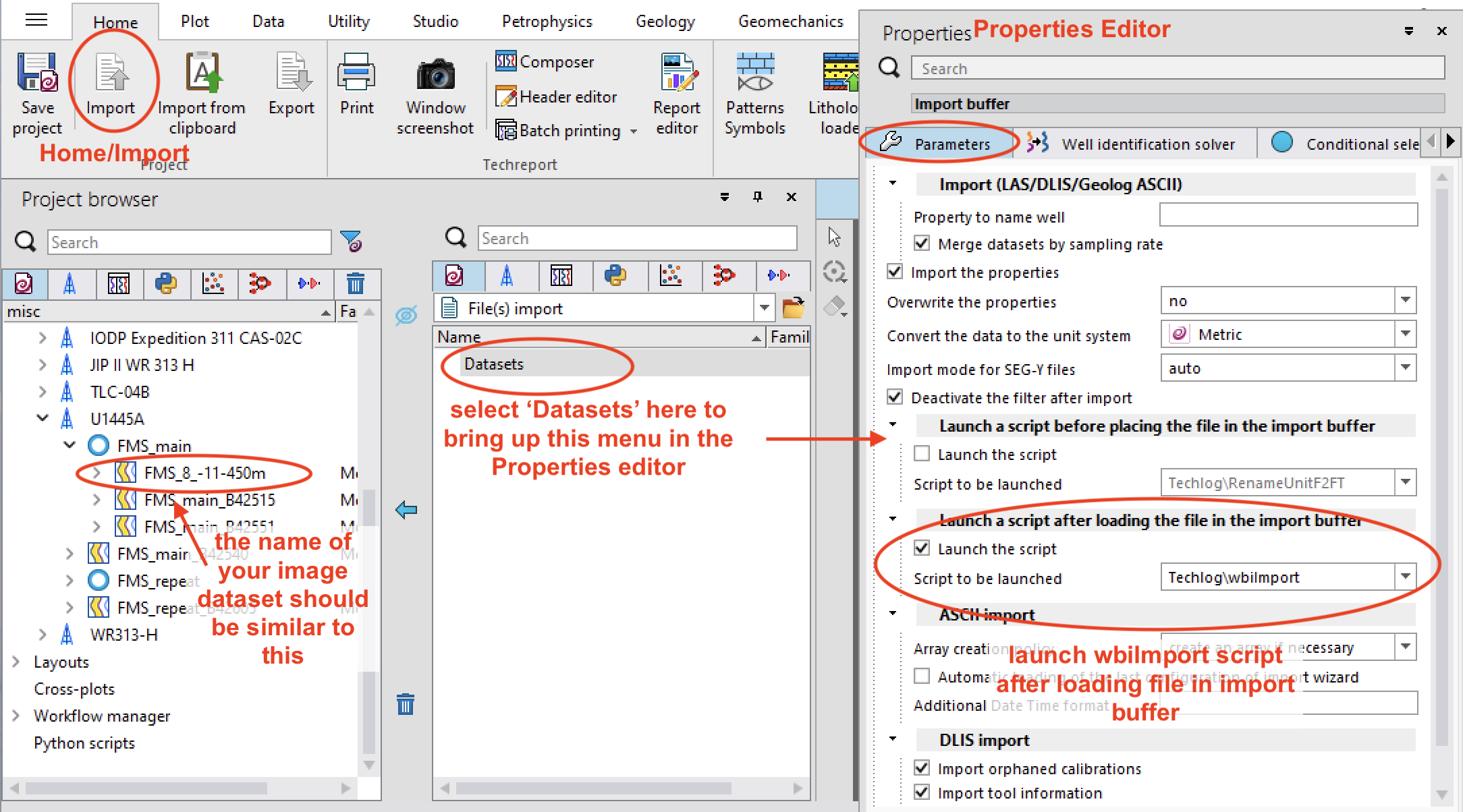
When importing FMS images that were processed with GeoFrame, it is necessary to
include the execution of a script in the importing process that will
group the variables necessary to generate the images into image
Datasets. After starting Home/Import, select 'Datasets' in the right
side of your import window, bring up the properties editor, select
'Launch the script' under 'Launch a script after loading the
file...', and select the 'wbilmport'.
Then import your file. This should create a dataset called
FMS_n_-xxx-xxxm - or similar, where n is 4 or 8,
depending on how Techlog recognizes the tool, and xxx-xxx is the top
and bottom of the interval logged, with 'ft' or 'm' at the end,
depending on the original field unit. This is the dataset that should be used
in the following steps.
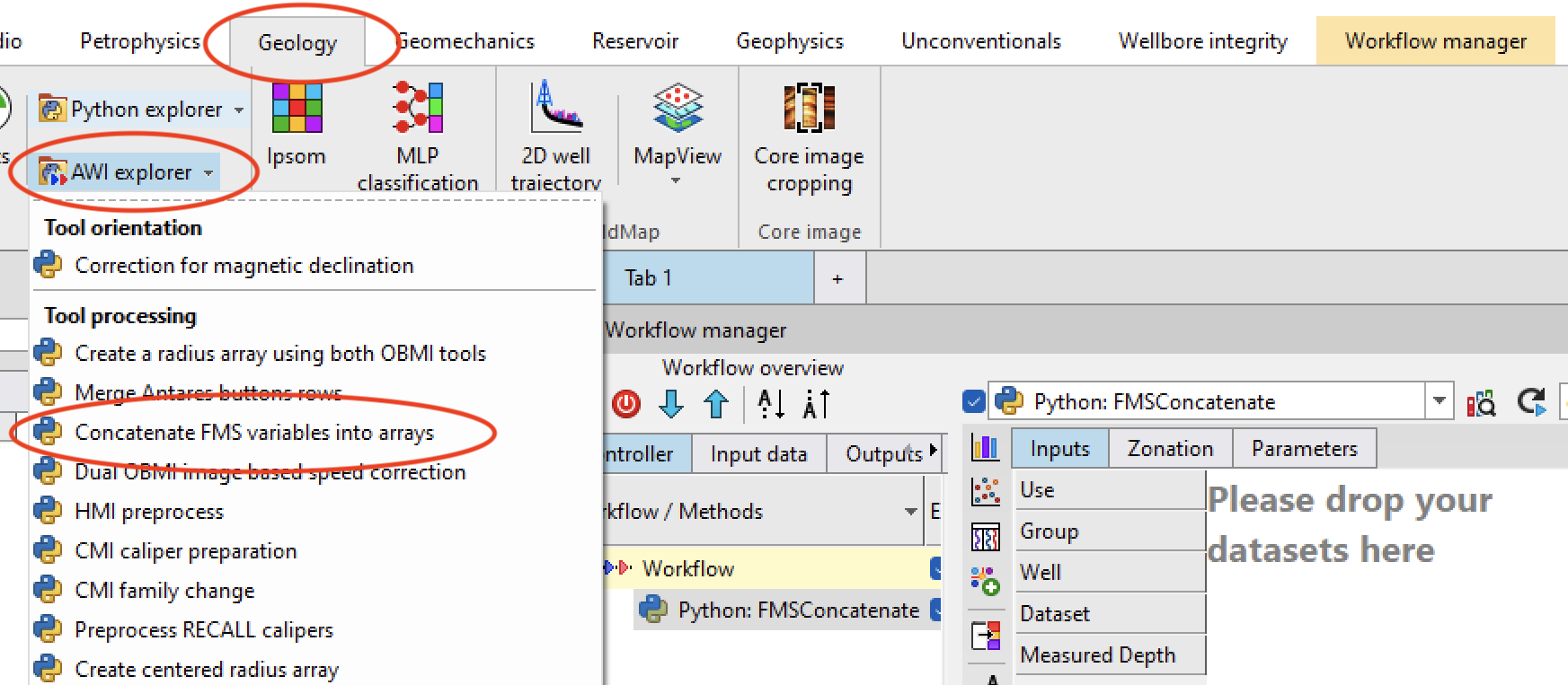
Concatenation of FMS variables
The FMS arrays are stored as individual buttons, that need to be regrouped into four pads.
Go into ‘Geology’/AWI explorer and select ‘concatenate the FMS variables into arrays’
This opens a small menu where you only need to select the hole that
you are working with.
Then select the image dataset and drop it where it says ‘Please drop
your data here’. The arrays are called BA11,…BA28,BB11,..BB28,..BD28.
This should create 8 arrays called
FCA1,FCA2,…FCD4 into your image data set, which correspond to the
two rows of buttons on each pad.
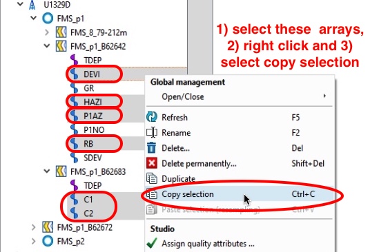
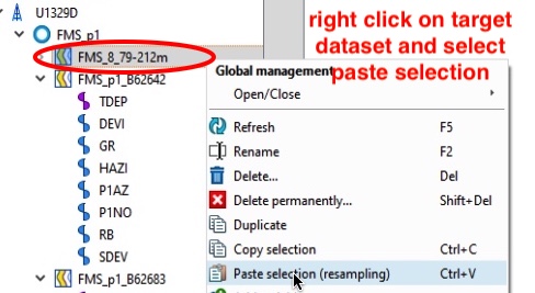
Before going further, you need to check if the orientation and
caliper arrays (RB, HAZI, P1AZ, DEVI, C1, C2) are already in the
same dataset as the button (BA11,…) and the newly created FC**
arrays. If they already exist you can skip this and proceed straight
to the Pad Image creation. If not, you need to copy these
arrays from the other datasets from the same pass.
Find these arrays (they may be in a DataSet with lower sampling
rate), copy them, one by one, or simultaneously with the control
key:
and then paste them into the FMS dataset:
A "resampling" window will appear (because the arrays have different
sampling rate than the FMS arrays) - select ‘Apply’ to proceed
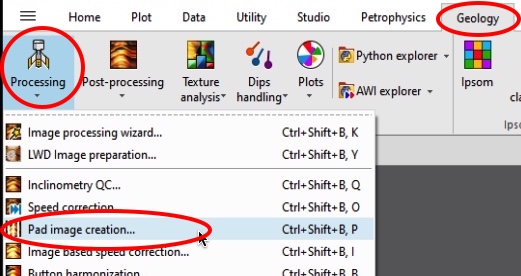
Pad Image Creation
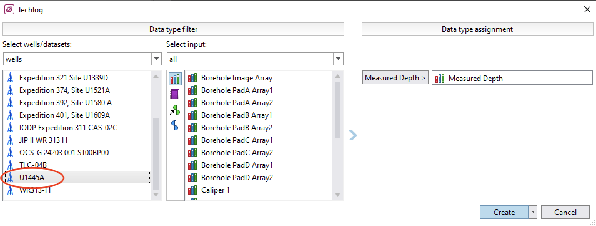
The next step is to group all the image arrays into 4 pads, one for each arm.
Go under Geology/Processing - and select Pad image creation
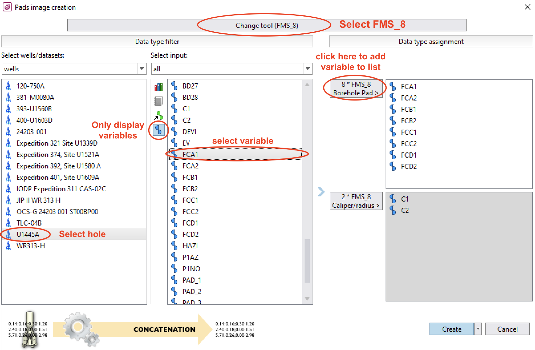
Here you have to select 'change tool' and change to FMS_8 (The ODP/IODP tool is actually FMS_4, but the option does not exist at this stage) and select the arrays to use.
To make the data assignment easier, select only your hole (if
there are other holes in the project), display only the variables
(blue icons), then select the correct variable, and click in the box
near the list of data to actually bring the data in any given list.
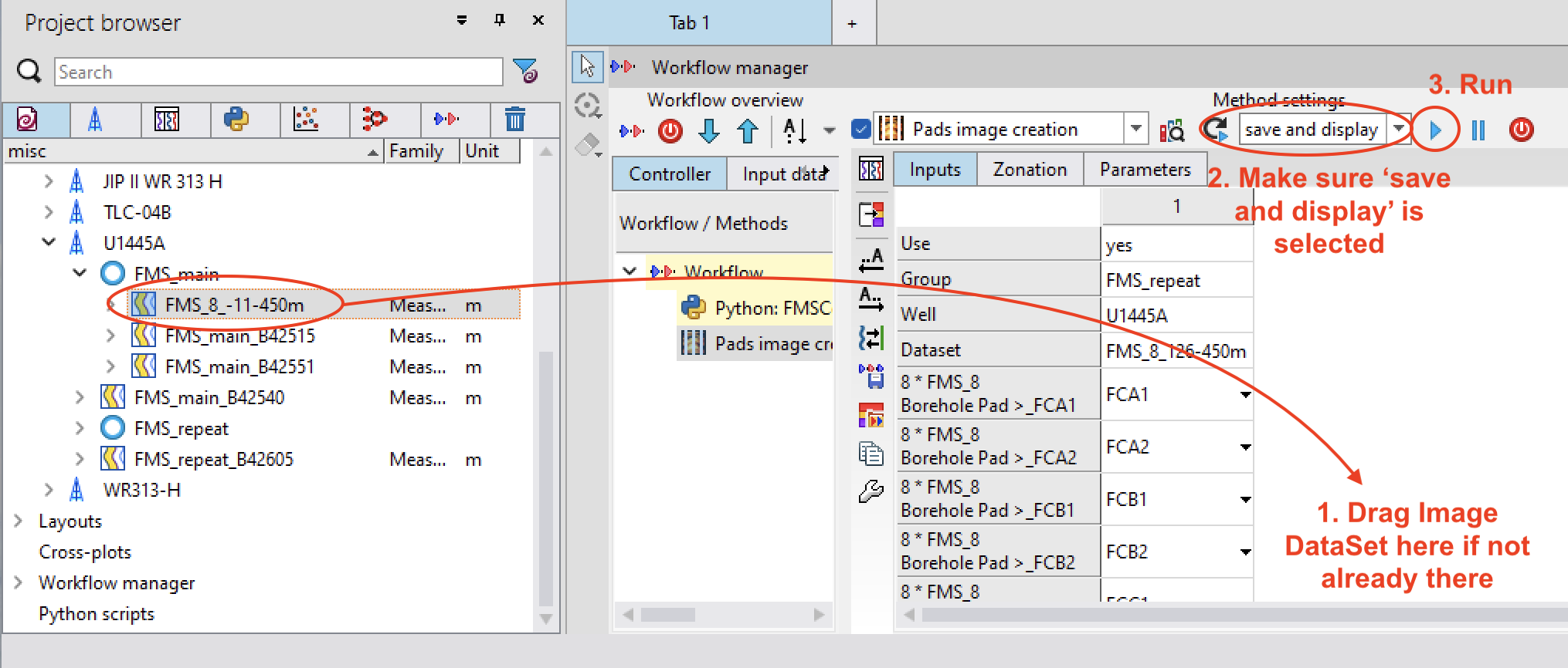
Then hit ‘create’ to close this window and initiate the workflow in
the main techlog window.
Make sure that the central menu says ‘save and display’, not just ‘display’, and hit the blue arrow to run the script
This creates the ‘PAD_*’ arrays, that still need to be combined with
orientation data to be displayed properly.
This is similar to the FMS processing results that you can find in
the LogDB processed dlis files that were processed with Techlog, and
still need one last step: the pad concatenation and orientation.
Data processed with Techlog (IODP Expedition 369 and later)
The image data processed with Techlog are already grouped into pads and need only to be concatenated and oriented.
When importing the dlis file (no need to run the Wbimport script), notice that all the auxiliary arrays that are not the pads (i.e. the azimuth, relative bearing, deviation,... all necessary to orient the images correctly) have a '_S' added to their name. This is the result of the 'speed correction' that was applied during the processing to correct for the motion of the tool during acquisition.
Except for this detail, the procedure for orientation and concatenation is the same as described below for data produced by GeoFrame
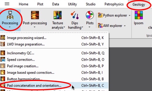
Pad Concatenation and orientation
Once created or imported, the pad image arrays need to be combined with the orientation data to be displayed properly and interpreted. In the
Geology/Processing menus, select ‘Pad concatenation and orientation’:
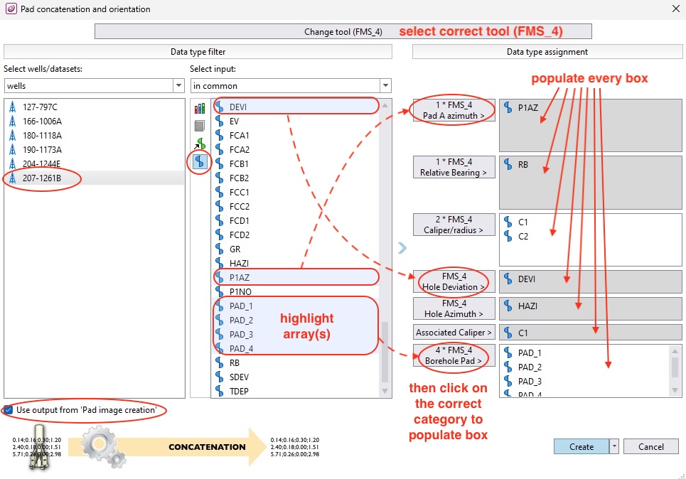
When the following window opens, you have to change the tool (select FMS_4), again display only the variables from your hole, populate every data type to the right with the correct array from your data set (with a '_S' for data from TechLog), and hit ‘create’. To add an array, say P1AZ, into the correct box, highlight the array, then click on the button near the box (i.e. 1*FMS_4 Pad A Azimuth for P1AZ).
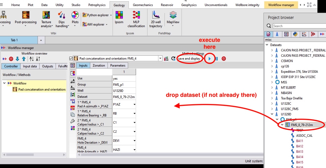
This opens the pad concatenation workflow in the main window. If you
have been through the array creation stages before, your Data Set is
already there and you just need to hit the blue ‘run’ button.
If you are just loading dlis data that were processed in TechLog,
select your dataset with FMS data, drop it in the window, then hit
run:
One more time, make sure that ‘save and display’ is selected before
hitting the blue arrow. This should complete the processing
and display an FMS image in your logview window. The new array will
have a name like ARRAY_WBI, which can be renamed more appropriately,
and that you can already display and interpret in LogView.
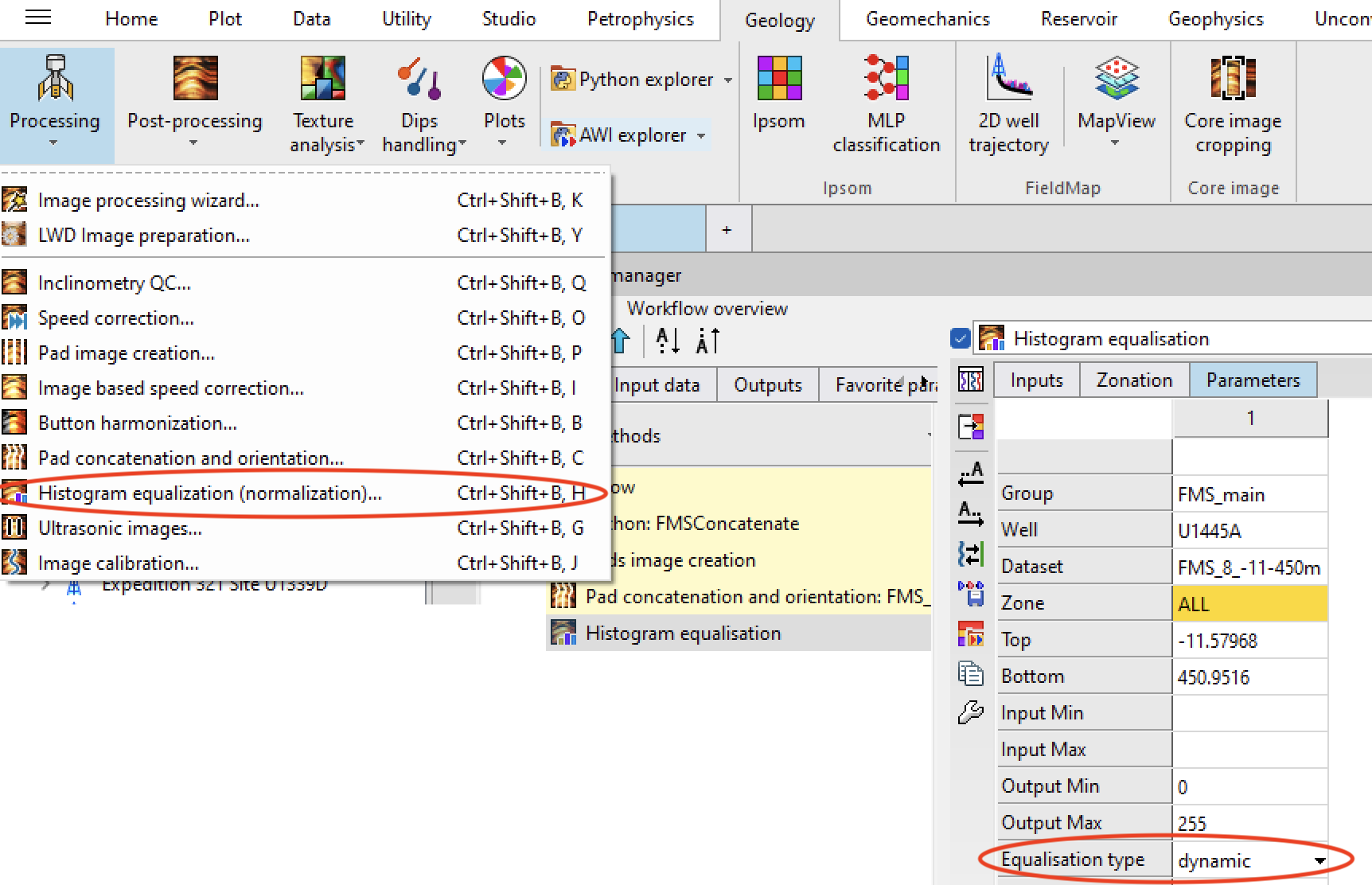
Image Normalization
One last step can be added to ensure that the images are similar to
the ones in LogDB: the ‘Histogram equalization’, or normalization,
which enhances the images and helps with the interpretation. Select
Geology/Processing/Histogram equalization (normalisation). Once
opened, you can choose either static or dynamic normalization:
static equalization is over the entire hole, for a broader
interpretation, while dynamic normalization is using a moving window
to enhance local contrasts.
One Final Note
Images displayed after this stage should look similar to the
LogDB gif images. One significant possible source of difference
is that in the creation of the gif images, a constant hole size
is assumed, to create images that cover about 25% of the hole.
The procedure described here uses the actual caliper, generating wider pads in
narrow intervals and thinner pads in enlarged intervals.