LogDB grd files

The LogDB images data are now available in netCDF/ grd format, a community standard for sharing scientific data, which is in particular familiar to users of GMT , the Generic Mapping Tools.
While the existing gif images already represent all the image data archived in the database, grd files deliver the same data in a more flexible format, allowing the creation of more personalized figures, the combination of several passes or tools, or the numerical analyzis of the data (statistics, spectral attributes, data masking, filtering,...).
The files can be read and displayed with NetCDF utilities or other tools, and one the most widely used tool is GMT, already used, for instance, in the LogDB plotting tool.
The following instructions describe the main steps to use GMT to produce figures in PDF format from any of these files. There are plenty of options to refine the figures, but those are the most basic steps.

File description
   - For all the imaging tools in LogDB (FMS, UBI, RAB, FMI, EcoScope - see our technology section for details on the tools), the data are stored as a 2D array covering the complete borehole wall along the interval logged: the horizontal (or x) axis is the azimuth, giving an "unwrapped" representation of the borehole wall, while the vertical axis (z) is the depth, at the same sampling rate as the original data.
   - In holes with multiples passes (typically for the FMS and UBI tool), there is one grd file for each pass of the tool.
   - All electrical image data (FMS, FMI, RAB) and the UBI ultrasonic amplitude images are normalized, using static or dynamic normalization, so the values are between 1 and 128 (or between 1 and 64, depending on when the original data were processed). Other files (radius from the UBI or various LWD data) include the actual measurement data.
   - For FMS or FMI data, where the coverage of the hole is not complete (these tools have four "pads" pushed against the borehole wall), the grd arrays were created for an ideal hole of constant diameter, assuming a 25% azimuthal coverage for the FMS tool, and 60% for the FMI. The values between the pads are flagged as NaN (not a number), allowing to ignore them when creating images. For these tools, the horizontal dimension of the 'straight' version, i.e. the image data without orientation but also without the space between the tool pads, is the number of 'buttons': 64 for the FMS, 192 for the FMI.
   - To display the most basic information on any of the files (such as the range for depth the image data or the sampling intervals), the most simple command is grdinfo.
   In GMT4 the command is just grdinfo
   In more recent versions of GMT, the command is gmt grdinfo
   For some basic statistics, add the -L1 option for median and L1 scale of z, and/or the -L2 option for mean, standard deviation, and rms.
   i.e. to extract the complete specs of the file 393-U1560B_1_stat.grd, the command is:
   grdinfo -L1 -L2 393-U1560B_1_stat.grd

In this specific example, some of the main informations displayed are the following:
   393-U1560B_1_stat.grd: Title: FMS data - Static Normalization - Pass 1
   393-U1560B_1_stat.grd: Grid file format: ns (#16) GMT netCDF format (short) (COARDS-compliant)
   393-U1560B_1_stat.grd: x_min: 0 x_max: 360 x_inc: 1.40625 name: Azimuth nx: 257
   393-U1560B_1_stat.grd: y_min: 127.345 y_max: 311.969 y_inc: 0.0025399 name: Depth (m) ny: 72688
   393-U1560B_1_stat.grd: z_min: 1 z_max: 128 name: Normalized FMS

Some explanations:
   • The FMS tool has four pads with 16 buttons each, i.e. 64 buttons total. Assuming that the pads cover 25% of the hole, the full width should be 256 bins per depth (with NaN to fill the gaps). Plus, to take into account the wrapping, one value is added, resulting in (nx=) 257 values for each depth depth.
   • The top and bottom of the interval logged (y values) are 127.345m and 311.969m, respectively, with a vertical sampling rate (y_inc) of 0.00254m (=2.54mm = 0.1in).
   • To be consistent with earlier versions of processing software, the nomalized values are from 1 to 128.

- To display some more information and actually extract all the values, used the ncdump command, which gets installed with the netCDF libraries when you install GMT. In this example, the following command:
   ncdump 393-U1560B_1_stat.grd > 393-U1560B_1_stat.txt
will create a text file with all the values in the grd file, which may be more convenient to import the data into other formats.

Color map
   - To create a figure, one can use any of the color maps that are part of GMT as cpt (color palette tables) files. To create an image with the traditional color scheme used for borehole images in many log interpretation software, you can download the following file: LogDB_img.cpt., and save it in the folder where you will be generating the figures (the grd files should also be stored in the same folder)

   - In GMT 4, to make sure that the color scale covers the range of the data, the following command must be used to create the color scale to use for the images. In GMT 5 or 6, this is done automatically when creating the image and this first step is necessary. So, for GMT 4 only, the following command will create the optimal color map called cmap.cpt for the file called 393-U1560B_1_stat.grd:
   grd2cpt 393-U1560B_1_stat.grd -CLogDB_img.cpt -Z -D > cmap.cpt

Creating a figure
   - To generate the figure, all you need to do is define its dimensions (height, width), the range of the image (the azimuthal coverage and the depth interval), and the spacing and position of the annotations.

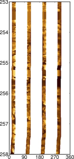
   - The following example shows how to create a figure with the FMS data from the file 393-U1560B_1_stat.grd, for the interval 253-258 m, with the full 360°, measuring 5 Inches vertically and 2 inches horizontally, with depth annoted every meter, and azimuth every 90°:
   In GMT 4, you need to produce first a PostScript file, then convert it into pdf.
   To create the postscript file, using the color table cmap.cpt that was created in the previous step:
   grdimage 393-U1560B_1_stat.grd -Ccmap.cpt -JX2i/-5i -Ba90/a1eWSn -R0/360/253/258 -Sn -Q > Figure1.ps
   Then to convert to the more versatile pdf format:
   ps2raster -Tf -A Figure1.ps

   In GMT 6, you can achieve the same result in one step:
   gmt grdimage 393-U1560B_1_stat.grd -CLogDB_img.cpt -JX2i/-5i -Bxa90 -Bya1 -R0/360/253/258 -nn -Q -pdf Figure1

Some explanations:
   • The option -JX2i/-5i, defines the dimensions of the figure (2 in x 5 in). The '-' for the vertical axis is to create a figure where depth (the vertical "y" unit) increases downward, as is standard when plotting borehole data.
   • The -Q option, necessary for FMS images, makes the values between the pads (NaN) transparent.
   • -Sn in GMT4 and -nn in GMT6 is to avoid interpolation between bins, and to use the value of the nearest bin. Otherwise the image can seem blurry or smeared.
   • The -Betc argument, slightly different between the versions of GMT, is used to define the spacing and layout of the labels.

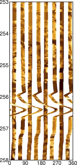
- The next example takes advantage of the new format to superimpose two FMS passes (files 393-U1560B_1_stat.grd and 393-U1560B_2_stat.grd) recorded in the same hole. When the arms of the tool don't follow the same track in the hole, it gives a chance for increase coverage of the borehole wall.

   In GMT 4:
   grdimage 393-U1560B_1_stat.grd -Ccmap.cpt -JX2i/-5i -R0/360/253/258 -Sn -Q -K > Figure2.ps
   grdimage 393-U1560B_2_stat.grd -Ccmap.cpt -JX2i/-5i -R0/360/253/258 -Ba90/a1eWSn -Sn -O -Q >> Figure2.ps
   ps2raster -Tf -A Figure2.ps

   In GMT 6:
   gmt begin Figure2
   gmt grdimage 393-U1560B_1_stat.grd -CLogDB_img.cpt -JX2i/-5i -R0/360/253/258 -nn -Q
   gmt grdimage 393-U1560B_2_stat.grd -CLogDB_img.cpt -JX2i/-5i -Bxa90 -Bya1 -R0/360/253/258 -nn -Q
   gmt end

Some more explanations:
   • In addition to the options described in the first example, GMT4 and more recent versions have different ways to build a figure in multiple steps.
   • In GMT4, all the commands except for the last one must include the '-K' option, to tell that other steps will be added to the postscript file. And every step except the first one must include the '-O' option, to recognize that it is adding to an existing postscript.
   • In GMT 6, gmt begin and gmt end are used to start and end a session. Every command between these two adds to the figure defined with gmt begin.
   • NB: in both cases, the annotation options -Betc needs to be used only once. It doesn't hurt to have it at every step, but the annotations just keep being repeated on top of each other.

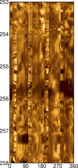
- The Final example also takes advantage of the new format to combine one FMS pass (files 393-U1560B_1_stat.grd) and one UBI pass recorded in the same hole. They are different measurements (conductivity vs. ultrasonic amplitude), but their combination can enhance the information provided by each image separately

   In GMT 4:
   grdimage 393-U1560B_amp_2_stat.grd -Ccmap.cpt -JX2i/-5i -R0/360/253/258 -Sn -Q -K > Figure3.ps
   grdimage 393-U1560B_1_stat.grd -Ccmap.cpt -JX2i/-5i -R0/360/253/258 -Ba90/a1eWSn -Sn -O -Q >> Figure3.ps
   ps2raster -Tf -A Figure3.ps

   In GMT 6:
   gmt begin Figure3
   gmt grdimage 393-U1560B_amp_2_stat.grd -CLogDB_img.cpt -JX2i/-5i -R0/360/253/258 -nn -Q
   gmt grdimage 393-U1560B_1_stat.grd -CLogDB_img.cpt -JX2i/-5i -Bxa90 -Bya1 -R0/360/253/258 -nn -Q
   gmt end

One last note:
   • The outcome of each command in GMT is "piled" on top of the existing results. So in this case, it was necessary to display the UBI image before the FMS image, otherwise the FMS pads would have been covered by the UBI image.

Resulting figures

Figure 1: FMS Pass 1	Figure 2: FMS passes 1 + 2	Figure 3: FMS pass 1 + UBI pass 2

These simple examples should give a sense on how to use and plot these data. GMT has been developed for various platforms, with various wrappers. These instructions were tested while using a terminal window on Linux or Mac OS, but should work with only minor adjustments for other platforms and/or distributions. For any question or suggestion, contact gilles guérin (guerin@ldeo.columbia.edu).