|
Instructions
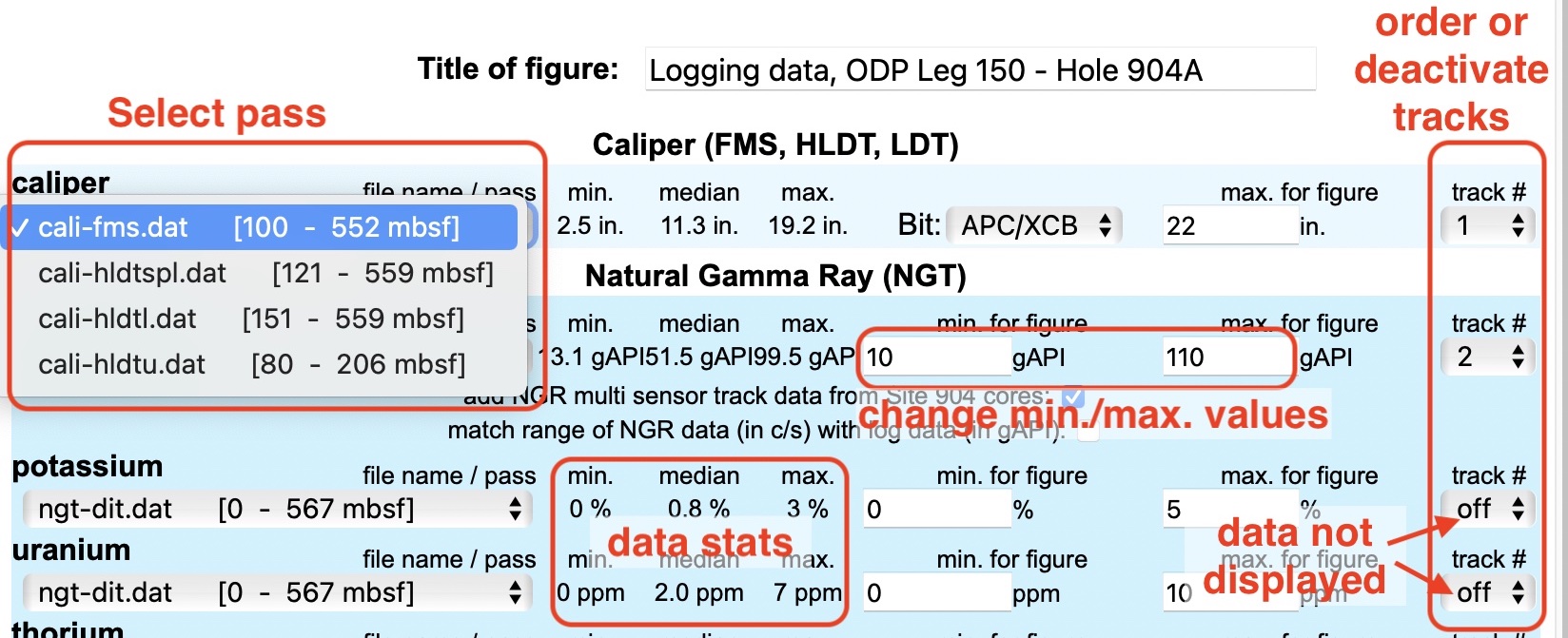
This is a utility to create a figure with the logging data from any hole in the LDEO Logging Database (logDB). Data are displayed in vertical 'tracks', as a function of depth below seafloor (mbsf, fbsf) or below surface (m,ft), depending on the oceanic or continental setting, and of the depth unit used in each program. The figure will be displayed in this frame, and these instructions can be displayed again in a new window through the link at the top of the page. The results are PDF files, that can be opened in any pdf/image viewer and edited (colors, lines, fonts,...) in any vector graphics software (illustrator, InkScape,...). The size of the figure, the order of the tracks (numbered from left to right) and their content is automatically preset to some default values, so without going further, you can click on 'create figure' at the bottom, without changing anything, to display the full scope of data for the hole. Here is a summary of some of the main options to adjust the figure to your needs: Selecting and ordering data and tracks The number of tracks, their order, dimensions and content can all be changed. The main choice is to define what data to display, and which pass for each data type. Logs are usually recorded in multiple 'passes', while lowering the tools in the hole (downlog, only some measurement), and, mainly, while pulling the tool up (uplog). Depending on hole conditions or operational factors, the data for some pass may be of better quality for some measurements, so it is important to look at all passes available. Only one pass can be displayed for any measurement, but you can chose which pass to display for each measurement. |
|
|
The names of the data files are based on the tool used and on the recording pass. If it is not explicit enough, use the file dictionary for each hole, accessible at the top of the page. For some data types (velocity in particular), there can be multiple channels to choose from. They appear with the file name in the file selection menu. Tracks can be reordered (numbered from left to right). The default (caliper then gamma ray on the left, which are the most common measurements) can be changed by changing track numbers, and turning 'off' some data. Only the number of the tracks matters - any gap in sequence will be shuffled left. The basic data statistics displayed (min, max, median value) can be used as a guide for the plot limits - adjust the values to enhance the variability in the interval you choose to display. NB: to reduce the possible influence of outliers created by the drill pipe or bad hole conditions, these values were calculated for 95% of the data for any data set. If there are no outliers, they may need to be adjusted to cover the full range of the data. |
|
|
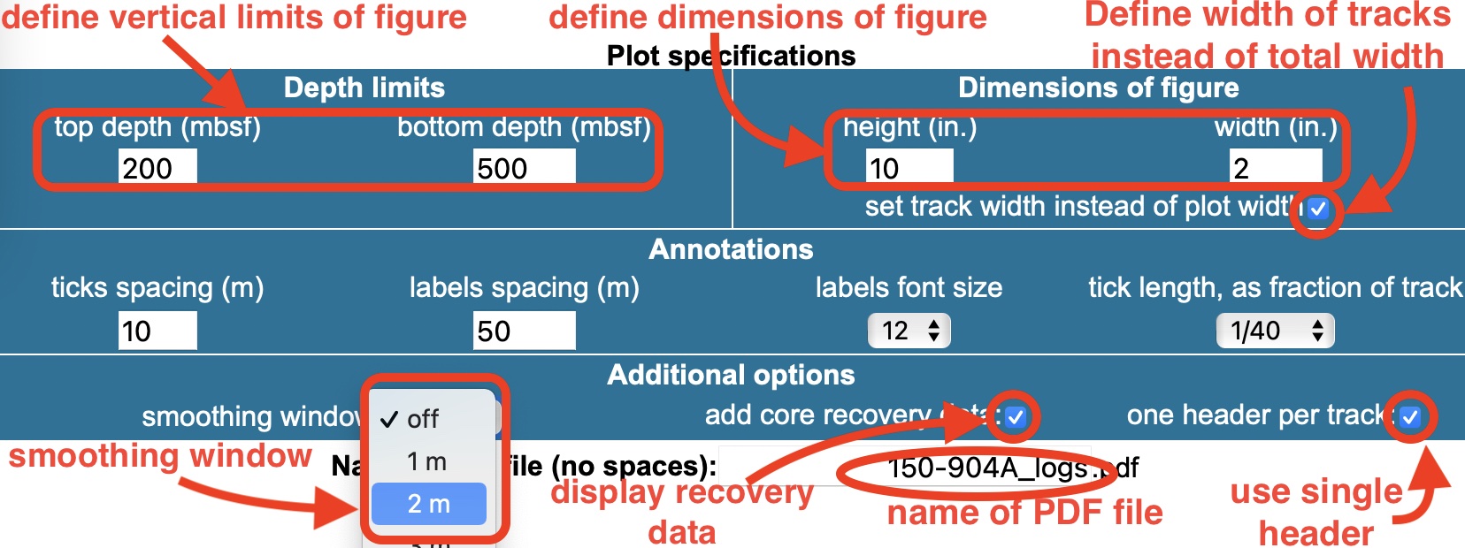
Display parameters The main parameters controling the appearance of the figure are defined at the bottom of the page, in particular the height and width of the figure. |
|
|
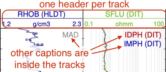
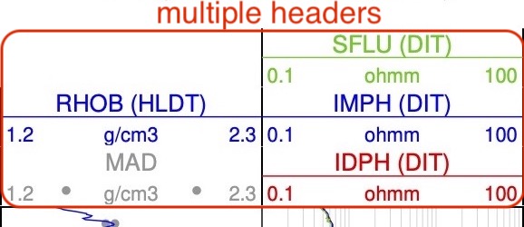
The default height is 10 inches if there are no image data (FMS, UBI, RAB,...), and 20 inches if image data exist for the hole. The default width is calculated assuming that each standard track (i.e. not image data) is 1.5 in. wide, and that image tracks are50% wider. You can either define the total width, or check the box under the width field to define the width of standard tracks. Image tracks are always 50% wider. You can also choose the spacing between the depth anotations and between the 'ticks' depth markers; the font size for the annotations; and the length of the ticks, which is defined as a fraction of the track. Negative tick length will display the ticks on the outside. And you can define the name of the pdf file that will be created and that you can download immediately. Additional options There are various options to include additional data or change the way data are displayed. When multiple curves are displayed in traditional logging 'blue prints' or 'field plots', all the captions and scales are piled on top of the track. Here, by default, only one curve is listed in the header, and other captions are inside the track. You can choose the traditional 'multiple headers' layout by unchecking the box for this purpose. |
 vs. vs.
|
|
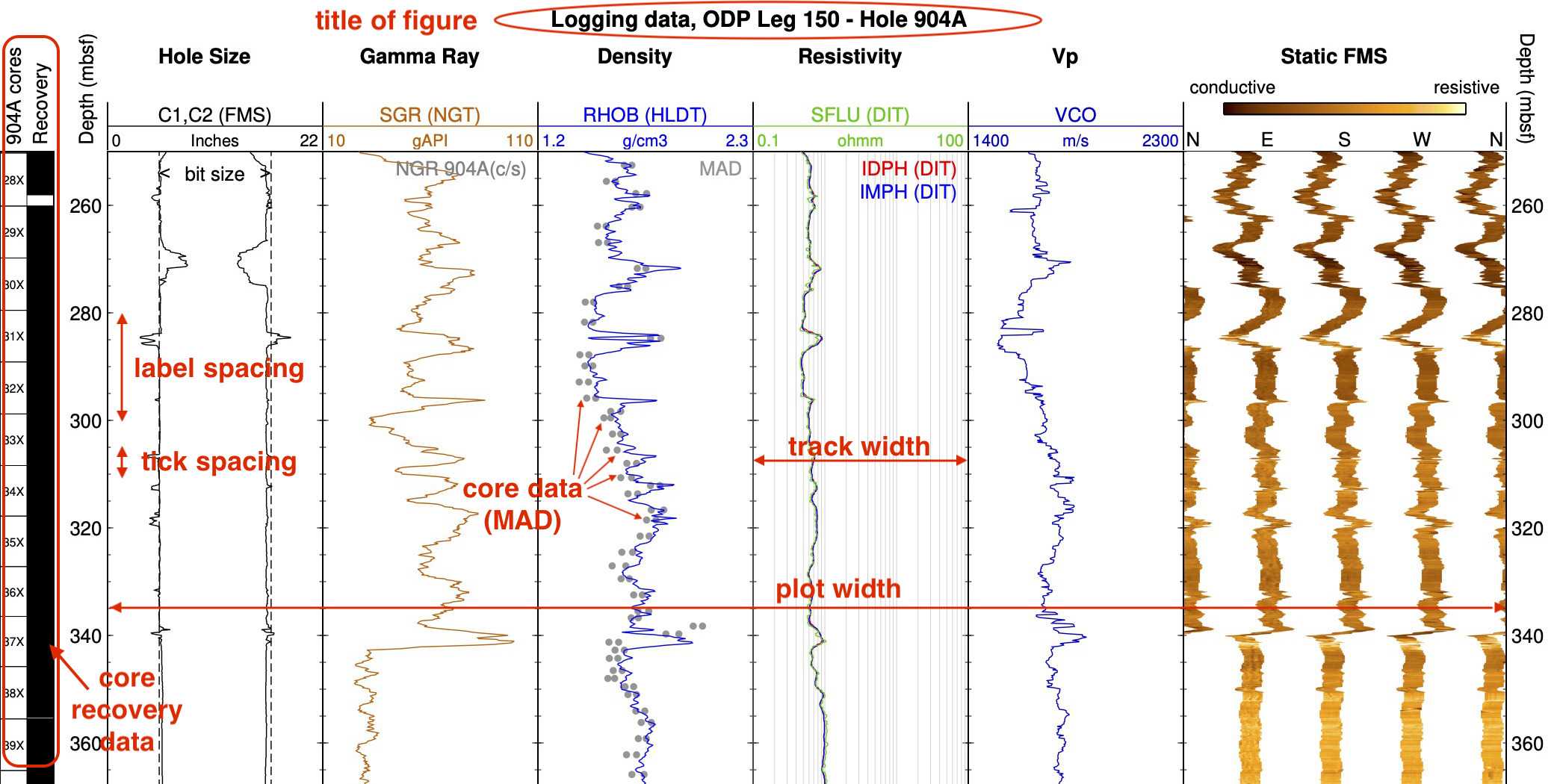
In some of the programs (ODP,IODP,DSDP,NGHP), some of the data measured on cores recovered from the same holes or sites can be added: gamma ray (from measurements on whole core sections), density and porosity (both from moisture and density (MAD) measurements on discrete samples). The unit used for gamma ray measurements on core is different from the gamma ray American Petroleum Industry unit (gAPI) of the logs, but you can choose to match the scales for better qualitative comparison. In holes from these programs, core recovery data can be added to the left of the figure for any hole where such data exist. To help assess the quality of the hole and of the data, the hole size (from caliper logs) is compared with the nominal hole size, which is the size of the bit used (dashed lines in the 'Hole Size' track). For most drilling programs, the value was known, but in some of the continental drilling programs it was only inferred from sometimes incomplete documentation. Also, for all DSDP/ODP/IODP, the default value is for an APC/XCB bit (piston coring). It needs to be changed to a RCB bit for holes drilled by rotary coring. If you don't know what bit was used but the core recovery data are available, you can find it from the core labels: rotary coring is indicated by cores ending in 'R' (1R,2R,...), while APC/XCB cores end with H or X (1H, 2H, 1X,...). Finally, you can apply a gaussian smoothing window to the data, and set the length of this window, in case the curves appear noisy for the scale and extent of your figure. |