5.1 Starting /closing IESX
5.1.1 Starting IESX
5.1.2 The IESX Session Manager
5.1.3 Closing IESX - saving sessions
5.2 The IESX data manager
5.2.1 Loading SEG-Y Seismic data
5.2.1.1 Loading 2D data
5.2.1.2 Loading 3D data
5.2.2 Loading Seismic Navigation data
5.2.3 Sharing seismic data between projects
5.3 Basemap - viewing the Navigation data
5.3.1 General features
5.3.2 Posting seismic surveys
5.3.3 Creating/Editing borehole sets and appearance
5.4 Seis2DV / Seis3DV - viewing and interpreting the Seismic sections
5.4.1 Viewing seismic lines
5.4.2 Creating/Editing vertical borehole appearance
5.4.3 Seismic interpretation (basics)
5.5 Synthetics
5.5.1 - Creating and adjusting synthetic seismograms
5.5.2 - Displaying synthetic seismograms and logs on a seismic line
5.6 Plotting
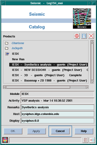
- One way to start IESX is to select in the 'Seismic' section of the product catalog in the Process Manager - and start it like any regular GeoFrame module. This will bring up the 'IESX Session Manager', from which you can start the various IESX applications.
- An other way to start the IESX Session manager is to choose the 'Seismic' icon in the 'Applications Manager': it will start the 'Seismic Catalog':
By clicking on the icon to the left of 'IESX', you can display previous sessions. A session can represent different kinds of data, different types of interpretations, different stages in a project, or only different ways to display things.5.1.2 The IESX Session manager
NB: The IESX sessions are associated with the activity (see Applications Manager). So make sure you have selected the right activity in the applications manager before starting the Seismic Catalog.
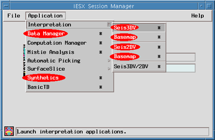
Pulling down the 'Application' menu displays all the IESX applications, among which the most commonly used are:5.1.3 Closing IESX - saving sessions
- IESX Data Manager (for loading, editing, sharing, deleting,... seismic data)
- Basemap (for viewing maps of the survey lines),
- Seis2DV / Seis3DV (for viewing and interpreting seismic data, and adding downhole log data),
- Synthetics (for generating synthetic seismograms).
Notes:
- If you have two monitors, you can choose on which monitor to open any of the IESX applications: press the 'Control' key while selecting the application - a window will popup asking on which monitor to open the new window.
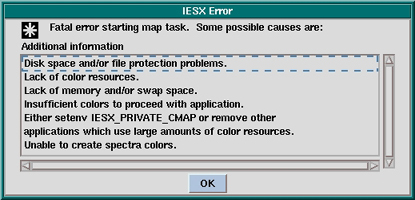
- GeoFrame applications - and IESX applications in particular - use up a lot of colors. Thus frequently, when starting any of the applications you may get the following error pop up (with some variations in the messages).The 'Fatal' in the message is a gross overstatement...
If you have only one monitor, it is almost impossible to have two IESX windows opened simultaneously (i.e. Seis2DV/3DV and basemap - the data manager is not a big color sucker). If you iconify the already open window (press the second button from right in the upper right corner of the window), you should be able to open the application - and then you have to juggle between the icons and the windows, iconifying one before restoring the other. To save color memory, exit all unnecessary windows: the Geonet window, the Project Manager, and any non-GeoFrame window.
A session will save not only what data were displayed when you saved it, but everything what was present in any IESX windows that were open when you saved it and the location/size of the windows in your screen. It is a convenient way to preserve particular configurations when working on a specific part of the survey, or on a specific type of interpretation or processing.5.2 The IESX Data Manager
To save a session: select 'File/Save as...' in the IESX Session Manager and enter the name of your session - or enter the name of your session in the area for this in the IESX Session Manager - and select 'File/Save' .
When you exit IESX, you don't need to exit from the individual applications. Exit from the IESX Session Manager, and you will be given the option to save the session one last time. The next time you open the IESX Session Manager, if you don't select a specific session, it will open the way you closed it the last time.
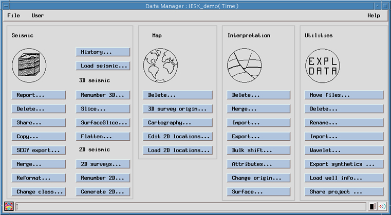
The IESX Data Manager allows you to import/export seismic data, to edit (delete, rename, copy...) seismic data, to share seismic data between projects and to export IESX-generated data such as synthetic seismogram, wavelets,....
To start it : Application/Data Manager in the IESX Session Manager:
Most command names are somewhat self explanatory, some are pretty obscure and not that useful - the most useful are:
'Report...' provides a general information summary for existing seismic volumes - the size, the sampling rate, number of samples, number of traces, some global statistics,... a quick way to check that all data were loaded.
'Delete...' - to delete classes of seismic data. A class is a version of seismic data, such as filtered, migrated, ...
'Share...' - to share seismic data between different projects and/or users - this can be very useful to save disk space, especially for large data sets.
'Load Seismic...' is the real piece of work to load SEG-Y seismic data.
'2D surveys...' - to move lines between 2D surveys.
'Load 2D locations' - to load navigation data which are necessary to locate your seismic data in space. In a perfect world, coordinates of the shot points should be in the headers of the SEG-Y files, and it would not be necessary to go through this step, but this is actually very rare. Navigation data should be in ASCII files made of columns with the line name, the shot point numbers and the coordinate of the shot points.
'Edit 2D locations...', 'Renumber 2D...', 'Renumber 3D...' can turn out to be useful if navigation data and seismic data do not have the same 'conventions' in the shot point and CDP numbers. They allow you either to 'correct' some locations or to renumber the CDP and shot points.In the 'Utilities', the most useful are 'Delete...' (seismic data can take a lot of disk space, and it can become necessary to remove unnecessary data - or data that were not loaded properly for some reason) and 'Export Synthetics' to save to ASCII files synthetic seismograms calculated in IESX .
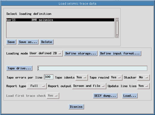
Start up `Load Seismic' from the IESX Data Manager:
- Create a Loading Definition by using `Save as...', and entering a name and description. The loading definition will save all the parameters required to describe and load your data. It can be used later to import data coming from the same source or with similar characteristics.
- Select the 'Loading Mode' - usually 'User defined 2D' for 2D data or 'User defined 3D' for 3D data.
- Before getting any further, it is usually a good idea to get a preview listing of the contents of the SEG-Y file. To this, select 'SEG-Y Dump...'
- Select the type of input storage (disk, tape,...)5.2.1.1 Loading 2D data
- If it's a file on a drive or CD-ROM, enter the full path to the SEG-Y data file.
- Set Trace Header to 'Full' to get the most complete overview of the headers.
- Limit the 'First trace' and 'Last trace' to a few traces (here 1 to 10) - you should get enough header information from the first shots.
- Select 'Sample' for 'Range Type' - and put a few samples only (here 1 to 5) - so it is going to list only the first 5 samples of each trace.
- Set 'Continue Prompt' to No - so it is not going to bug you every page.
- Select 'File' as output media - and give a name (with it's full path) to the text file to be created. This will allow you to open this description file in a text editor and have it open for reference while filling the input specifications
- press `Dump...'.
-> 'Dismiss' to close
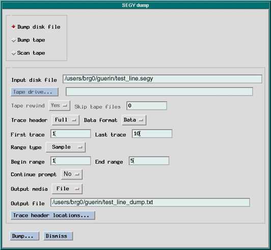
The ASCII file produced will contain a description of the different headers in the SEG-Y file:
- Reel Header - General information about the file. EBCDIC format. 3200 bytes.
- Binary Reel Header - 400 bytes.
- Trace 1: binary header - 240 bytes
trace data - generally 32-bits IBM or IEEE floating point format- Trace 2: binary header - 240 bytes
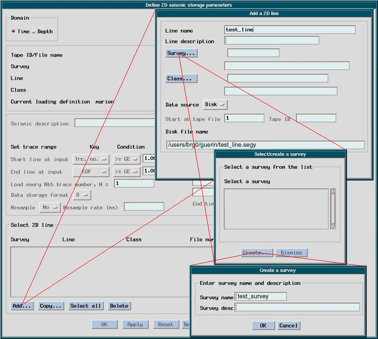
trace data,...etc.- Back in the 'Load seismic trace data' window, select 'User defined 2D' and press `Define Storage...' to bring up the 'Define 2D seismic storage parameters' window:
Note: this figure also illustrates that the different steps in this definition can bring up a lot of successive windows. It might happen that things appear frozen or that you can't dismiss one of these windows only because the latest small window is hidden behind some other one. This can happen here, or during the 'dumping' or in later steps - windows have to be closed in the reversed order they were open.
- Press `Add...' to bring up the `Add a 2D line' window.
- Enter the line name.
NB This must be the same exact name (case and all) as in the navigation data file (see loading navigation data)!
- As in the figure above select/create a Survey... and a Class....
- Select the type of data storage (`Disk' or 'Tape') and enter the full path name or tape device name.
- Once the survey/class and file names are defined, they appear in the 'Define 2D Seismic storage parameters' window.
- In order to save space or to focus your data, you can also use this window to define the first and last trace(s) to load, a trace subsampling rate, and/or the times to end/stop trace loading (for instance to remove the water - or the deepest part).
- Click OK to close the window.
NB you may want to use similar parameters to load additional seismic lines - and the 'copy...' function will help doing that, but it is best to define the SEG-Y input format before pressing `Copy...' to set up the other lines (you only have to enter the input format once this way).
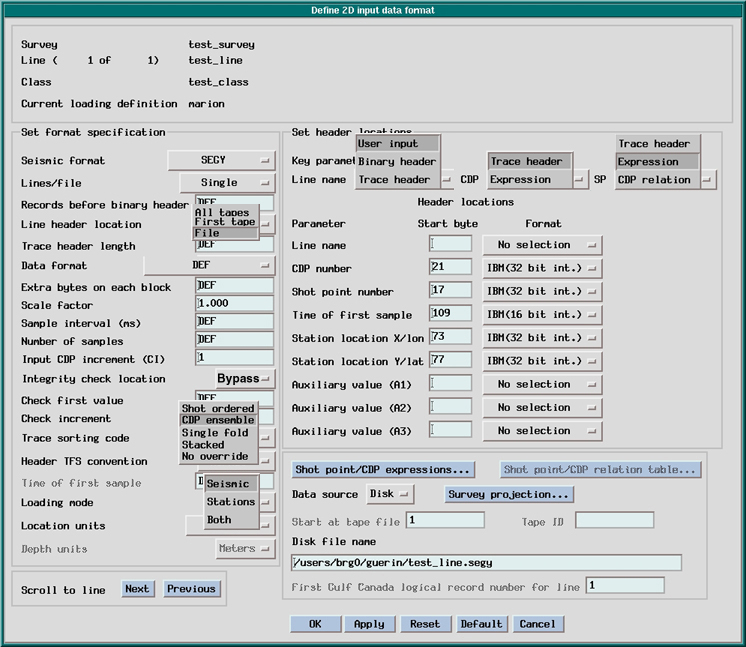
- Press `Define Input Format' in the 'Load Seismic Trace data' window to start to 'Define 2D input data format' - which is used to define the format of your SEG-Y file. Because the SEG-Y format is highly flexible, it is most likely that you will have to change some of the parameters in this window. To do this, it is useful to open the ASCII file with the results of your SEG-Y dump in a text editor.
The most current parameters to check and/or change are:
In the 'Set format specification' area (general description of the structure of the file):
- Specify if you have one 'Single' line or 'Multiple' line per file
- Specify where the general line (reel) header is - most likely 'File' or 'First Tape'.
- You will want to 'Bypass' the integrity check location.
- The trace sorting code is the order of the records in the file. Usually CDP ensemble (this can be deduced from the order in your SEG-Y dump).
- The loading mode is either 'Seismic' if you have a separate file with the navigation data or 'Both' (meaning seismic and navigation (stations)) in the rare case where shot point locations are present in the trace headers. In this case, you have to select the 'location units' (meters, feet or lat/long, depending on the nature of the navigation data)In the 'Set header locations' area, you specify where the information on line name and CDP and shot points (SP) numbers are taken.
- The line name is usually defined by 'User Input' - it will assign the line name that you have previously defined. However, in particular when multiple lines are in one single SEG-Y file, it might be necessary to get the line name from the 'Trace header' or the 'Binary header'. This should be apparent in the SEG-Y dump file.
- The CDP number is usually taken in the trace header - look in the SEG-Y dump for 'CDP ensemble' or 'CDP trace number'. However, in rare occasions, it might be necessary to define an 'Expression' based on trace number or other factors.
- The SP (shot point) number has pretty much as much chance to be in the 'Trace header' as to have to been defined by an 'Expression'.
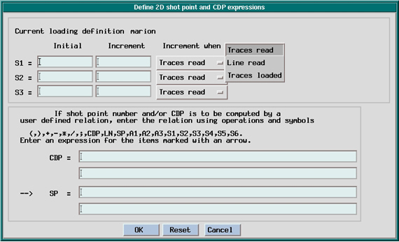
- The default values and format for the header locations are often correct - but still need to be compared with the SEG-Y dump file. This is necessary for any of the file name, CDP or SP that are to be found in the 'Trace header'. If you have chosen 'Both' in the loading mode (i.e. loading seismic and navigation data), you also have to make sure that the station locations (X,Y) are pointing to the correct header location.Defining an expression for CDP and/or SP: select 'Shot point/CDP expressions...' to pop up the following window (this is a 'condensed' version of the actual window).
In the most common case, you just have to define an expression for SP as a function of CDP (SP = CDP, or SP=5*CDP+100, ...).
In more exceptional cases, where neither CDP or SP numbers are in the trace header, you have to build the expression from scratch - and use the 'S1','S2',...'S6' variable for this. For instance, if you know that your first CDP number is 1023 and that each trace in the file is a new CDP, you can define:
Initial S1 = 1023 - S1 Increment = 1 - S1 increment when 'Traces loaded' - and CDP = S1.
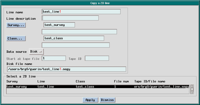
'OK' when doneIf you have additional lines/files to load that were stored in a similar manner, return to the 'Define 2D seismic storage parameters' window, select (highlight) the line you have just defined and press `Copy...' to bring up the 'Copy a 2D line' window:
In this example we just change the line name, and the disk file name (changes in red).
Don't forget to 'Apply' for each new line
'Dismiss' when finished.In the main `Load seismic trace data' window, press `Load'. A window will pop up saying the input parameters are OK (or not), and prompt you to continue. Information on the lines being loaded will be displayed on the screen. A message will announce that the loading is finished, but the time clock will continue to run, and the CPU will apparently still be working at full rate. This is a bug in the program, and you can safely close the Load Seismic application at this point.
You don't need to load the navigation data to view your seismic lines - at this stage, it can be useful to start 'Seis2DV' or 'Seis3DV' to visualize your data and make sure that the loading was successful
- In the 'Load seismic trace data' window, select 'User defined 3D' as loading mode, and press `Define Storage...' to bring up the 'Define 3D seismic storage parameters' window:
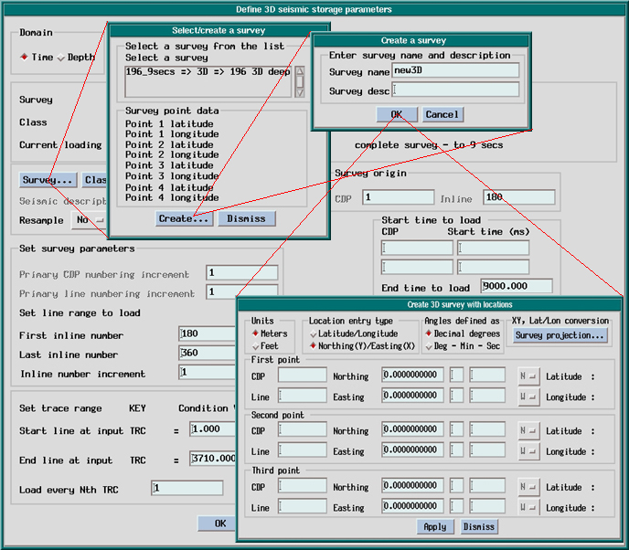
The procedure is very similar to the 2D loading, using a SEG-Y dump to determine the location of the headers. The most significant addition is the requirement to enter the coordinates of three points of the survey. This is shown in the above figure - clicking 'Survey...' pops up a Select/create survey' window were the coordinates of the 'corners' should appear. For a new survey, there is initially no value - you have to 'create..' the new survey - give it a name - then 'OK' to enter the coordinates of the 3 points. In the 'create 3D survey with locations' window, the 'CDP' number is equivalent to crossline number, and the 'Line' number is the inline number.5.2.2 Loading Navigation data
In the 'Define 3D seismic storage parameters' window, you have to enter the first and last inline numbers, the CDP (crossline) and inline numbers at the origin, the length of the lines (inlines), and eventually a subsampling rate. You can also specify the minimum and maximum time to load, to remove some of the sea and/or the deepest reaches of the survey.
The navigation data files should be space delimited and formatted into columns. It should contain the name of the seismic line, the shotpoint number, and the coordinates (latitude and longitude or X and Y using the same convention as defined when creating your project)
All the lines in the survey can be concatenated in the same file.- Start up `Load 2D Locations' from the IESX Data Manager:
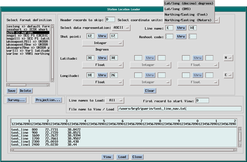
- Enter the full path to the navigation file, and press `View' to display it in the lower window. The numbers in this window indicate the column numbers to help describe the structure of the file (the upper row gives the multiple of 10).
- Select the coordinate units system: the most frequent are `Lat/Long (decimal degrees)', and `Lat/Long (DMS - Degrees, Minute, Seconds)'
- Enter the position in the records of the Line Name, Shot Point, Latitude and Longitude. If the coordinates are in DMS (degree, minute, second), you will have to enter also he position of the minutes and seconds.
- Select N/S and E/W. (North and East are positive latitudes and longitudes).
- Press `Survey...' and select your survey.
- Press `Save', and enter a format definition, to save these parameters that might have to be reused or edited if there is a mistake or a later changes.
- Press 'Load' - then 'Close' if successful. You will be able to visualize the navigation in the basemap
In order to save disk space and to avoid loading twice the same data set, it is possible to access seismic data from other projects
To do this, select 'Share...' in the IESX Data Manager to start the 'Share Manager':
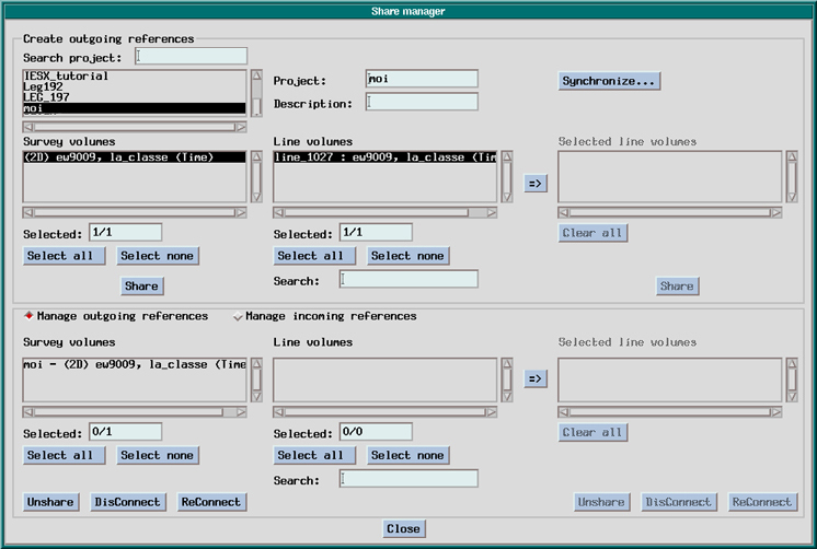
The 'outgoing reference' actually designates data from other projects that you want to access from your project. The list in the upper left corner shows all the project present in the same Oracle database server. When you select one, you are prompted for the password to this project. The survey volumes present in this project will then appear - selecting one will display the seismic line present,...5.3 Basemap - viewing the Navigation data
-> select the items you want to access - and 'Share'.
This operation can take a while if it's a large data set.The lower section is for managing shared items - it is used mostly to 'unshare' some items so that they can be deleted. Any shared items cannot be deleted, so you have to unshare it before deletion.
Start Basemap from the applications/Interpretation menu in the IESX Session Manager.
- The first time you start it, navigation data of the last survey that
you have just loaded should be the only thing to appear by default.
- You can then select what survey and what borehole(s) to display.
- Whenever your cursor is on (or close to) a line, this line will be
highlighted (here in cyan), and in the bottom message areas you will see
the line name, the survey name and the shot point and CDP numbers the closest
to your cursor.
- If you have a Seis2DV or seis3DV window opened, the seismic section
currently displayed in this window will be highlighted in the basemap (here
in red).
- You can define general attributes such as background color, highlight
colors, scale location, ticks... under User/Map Annotations.
- When a line is highlighted, MB3 will popup a menu with several
possible actions. The most useful are:
- Conflict: it can happen that there is an ambiguity in the line
selection (lines too close, multiple lines using the same navigation data,...).
In this case, 'conflict' will appear bold, and by selecting it you will
have to choose which line you want.
- Inline/crossline : this is mostly useful with 3D surveys - selecting
one or the other will define what lines get highlighted when you navigate
the map with your cursor.
- You can choose to save any configuration of
boreholes/surveys displayed as a 'Map' by selecting 'File/Save as...'
. You will be able later to recover this configuration with File/Open....
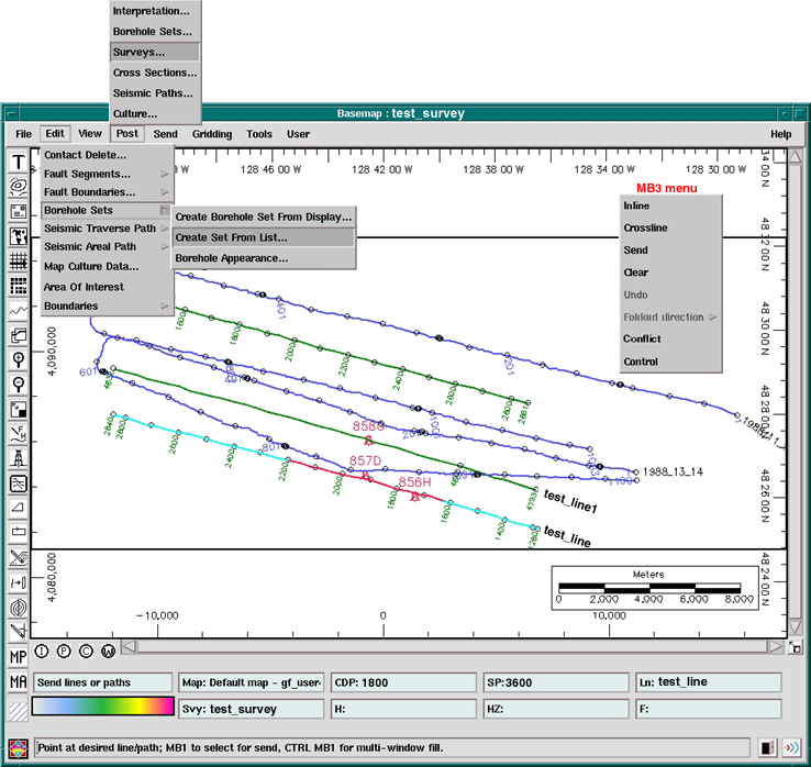
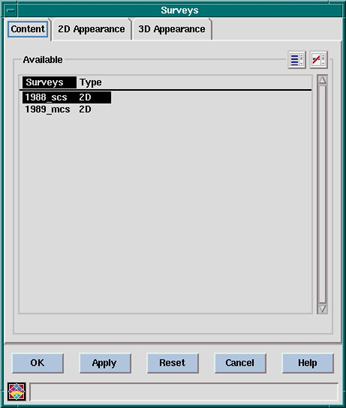
5.3.2 Posting seismic surveysIf you have multiple surveys, you can choose which one(s) to display - by default only the last one loaded will appear.
To add or remove surveys select 'Post/Surveys...' to bring up the 'Surveys' manager:
 |
 |
In the 'Content' menu (left), you select the survey(s) to display (press the 'Control' key to select multiple surveys).
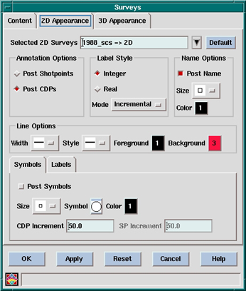
In the 2D/3D appearance (right), you define the general appearance of the survey: color, symbols/labels to be displayed
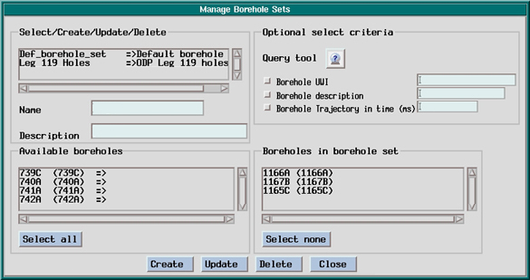
5.3.3 Creating/Editing borehole sets and appearanceTo display boreholes, you have to create 'borehole sets', and then 'post' the borehole sets.
A 'borehole set' is a group of boreholes that will have a common 'appearance' - typical borehole sets are holes from the same leg (in the case of multiple legs in one location), or proposed holes vs. actual holes, or whatever grouping is appropriate to the situation.
The same borehole sets are also used in the Seis2DV/Seis3DV applications, and can be edited/created from these applications.To create a borehole set:
- From Basemap: 'Edit/Borehole sets/Create from list... to start 'Manage borehole sets' window:
(In Seis2DV and Seis3DV use 'Define/Borehole set...' for the same purpose)
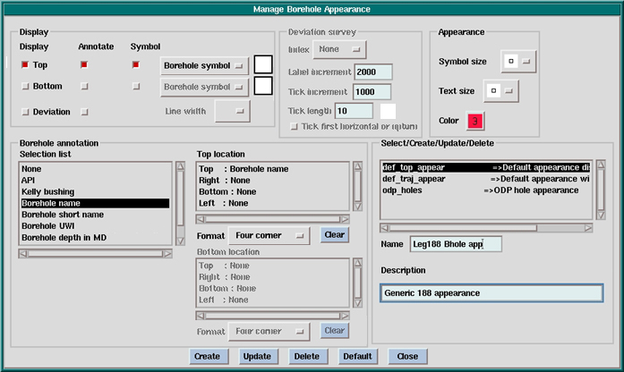
5.4 Seis2DV/Seis3DV - viewing and interpreting seismic sections- Choose the boreholes from 'Available boreholes' - they will move to 'Boreholes in borehole set'To be able to display a borehole set, you have to define an 'appearance' for it: use 'Edit/Borehole Sets/ Borehole appearance...' in the basemap:
- To remove boreholes from a set, select in 'Boreholes in borehole set' and it will move back to 'Available boreholes'.
- Name the set (e.g. Leg_119_holes).
- 'Create' (if it's the first time) or 'Update' if you are editing an existing set.
->CloseDefine the parameters for the appearance (size/color), eventually a symbol, give a name, then 'create' or 'update' (if editing an existing appearance).
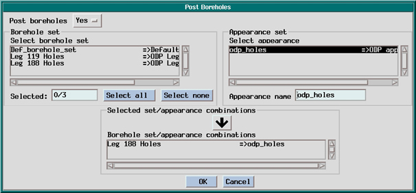
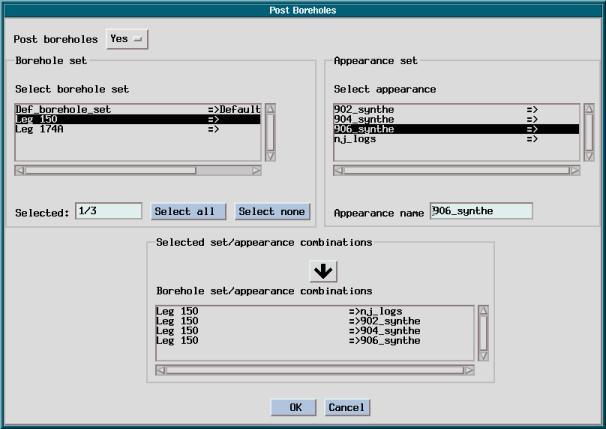
To post the boreholes on the map, use 'Post / Borehole Sets':
Select the borehole set you want to display and the appearance you have defined, then hit the arrow to make the borehole set and the appearance you have selected appear in the 'Selected set/appearance combinations' area.
-> 'OK' to apply and close.
5.4.1 Viewing seismic lines / general features
Seis2DV/Seis3DV are the applications used to visualize and interpret seismic lines. To start them, select Application/Interpretation/Seis2DV (or Application/Interpretation/Seis3DV) in the IESX Session Manager:
- The application will open with the first seismic data in the list. To change it to the line you want, use Display Menu / Seismic Line, and choose the survey, then the line from the list.5.5 Synthetics
- If you have a basemap opened, you can select the line you want to display in Seis2DV/3DV by selecting it on the basemap. The line will appear highlighted in the basemap (default in yellow), and the section actually displayed will be highlighted in a different color (default red).
- To change the colors, or to change to a `wiggle' display, use the Define Menu / Display spec, and change the Display Style: VI = colors, VA = wiggles. To cycle through the color options, press the color bar at the base of the window. There is also a VI/VA toggle at the base of the window.
- To change the scale, use Define Menu / Scales, and then set the trace decimation, the horizontal scale (traces per inch) and the vertical scale (inches per second).
- Use the magnifying glass icons for zooming in and out.
- As your cursor navigates the window, the message area displays the trace and CDP numbers and the two-way travel time.
- Where two seismic lines cross, you can have a `Foldout' to display the intersection of the lines (use Display / Fold vertical).
- To display any two or more seismic lines on the screen at the same time, use Define / Layout.
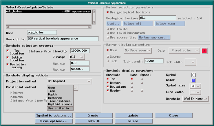
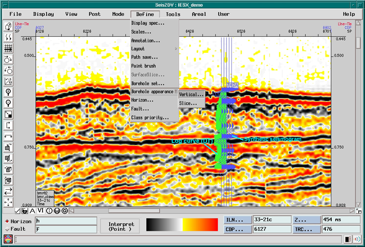
5.4.2 Creating/Editing vertical borehole appearance
- The Borehole sets defined in basemap are also valid in Seis2DV/Seis3DV. New sets can also be created or existing sets can be edited in the same way as described for basemap from Define/ Borehole Set.
- Before posting boreholes, you have to define a vertical borehole appearance (like in basemap). To do it, select 'Borehole Appearance/Vertical...' in the 'Define' menu (see figure):The main parameters to define in this menu are:
- The name of the appearance that you are about to create or edit.
- The maximum distance between a borehole and a seismic line for the borehole to appear in Seis2DV. This distance is defined in the 'Distance from line' area. From the basemap, you can figure what is the actual distance between wells and lines, and use it for your criteria. Choose 'Use criteria' as constraint method in the 'Borehole display methods'.NB: the distance between a well and a line is the shortest distance between the well and the line - i.e. the distance between the well and it's orthogonal projection on the line if you use the orthogonal projection method.
- General display parameters such as symbol, color, annotations.
- You can choose to display log curves (maximum two logs - one on each side of the trajectory) and/or synthetic seismograms. To do this, select 'Curve options...' and/or 'Synthetic options...', respectively.
NB: - if two curves with the same code exit for a borehole (ex: RHOB,...) only the most recently edited will appear.
- IESX recognizes only a limited amount of curve names. Make sure the curve you want to display has such a name.
- To be able to display a log along a borehole, you must have a checkshot survey for this borehole.
- To apply your parameters, press 'Create' or 'Update' (whether you are creating or editing an appearance)
-> then 'close' to get back to the Seis2DV display.
- To post the boreholes, the procedure is similar as in basemap: select 'Post/Boreholes...' to bring up a 'Post Boreholes' window identical to the one in basemap. Select the borehole set(s), the vertical appearance that you have defined, press the arrow to validate your selection - and 'OK' to close.
- Once a well is displayed, you can double click on its label to bring up the 'borehole editor' and change/edit the checkshot survey, reference depth or any other attribute:
- To change the checkshot, select 'Checkshot survey...' to start the 'Select preferred checkshot survey' window, and select the appropriate checkshot. 'Apply' to update the seismic display without closing your window - or 'OK' if you want to close.
- To edit the checkshot, double-click on it in the 'Select preferred checkshot survey' window.
- To define where the borehole label will appear on the seismic line: change the two-way time to the value where you want the label to appear (if the seafloor is at 1 second, you might want to put the label at 0.9 sec). If this first line is (0,0), the label appears at the top of the Seis2DV/Seis3DV window - change the 0 in the two-way time column to where you want the label. If the first value is actually the top of your logged interval, the label will be just at the top of the synthetic/log - in this case, you have first to 'add a line' at the beginning of the survey, and enter where you want the label to appear - and put '0' in the depth column.5.4.3 Seismic Interpretation - Picking Horizons/faults.
- Define / Horizon will bring up the Horizon Manager. Give the new horizon a name (e.g. top_sand) and a color. Add (or Update if you made changes to an existing horizon).
- Use the items in the Mode menu to define your actions: erase, snap, or smooth a horizon.
- On the seismic, choose `H list' from the right mouse button (MB3) menu, and select the new horizon.
- Pick the horizon point by point on the seismic with the left mouse button. Use Undo from the MB3 menu if you make an error.
- Choose `Break' from the MB3 menu when finished.
- Use Post / Interpretation to control which horizons are displayed on the seismic.Faults work in the same way as horizons.
5.5.1 Creating and adjusting a synthetic seismogram
The basic idea behind creating a synthetic is to line up the reflections that we expect the formations to create (the synthetic) to the reflections in the seismic data. The seismic can then be interpreted in terms of the actual formations, and, conversely, you can find out how deep into the seismic the borehole penetrated.5.6 Plotting
A seismic trace can be simulated in 1D by the convolution of a wavelet (representing the seismic source) and of a reflection coefficient series calculated by impedance contrasts downhole, which can be calculated by a sonic and a density log.
To start, select Applications/Synthetics in the IESX Session Manager.
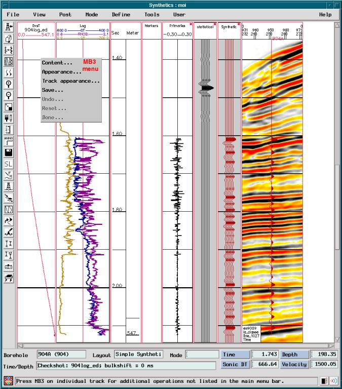
When you open this window for the first time, the latest DT log of the latest edited borehole will appear in the 'Log' track. A first estimate of reflection coefficients (Primaries) computed from this sonic log will appear in the 'Primaries' track -and a synthetic seismogram will be in the 'Synthetic' track, calculated by convolution of this 'primary' and of some default wavelet.This figure shows the Synthetics window after all the steps below have been completed.
- To modify the content in any track, select 'MB3/Track content...'.
- To modify the appearance in any track (colors, scales), select 'MB3/Track appearance...'.- To select another borehole, use File/ Open Borehole from list..., and choose one of the boreholes. The layout should be `Simple Synthetic' by default.
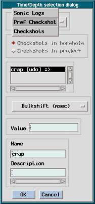
- By default, the 'Depth vs. time curve' in the DvsT track (left) is calculated from the last edited slowness log. If you have loaded checkshots, or if you have previously defined a depth vs. time relationship, you can change the content of this track with 'MB3/Content...':
Here you can select what kind of time/depth conversion to use (sonic log or checkshots), and what curve. You can also define a value for a "vertical bulkshift", but this can be done later more accurately with the interactive Mode/Bulkshift option. As soon as you select your conversion curve and close this window, the synthetic will be recalculated, and the synthetic display updated.
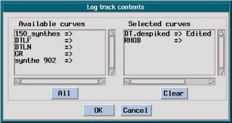
- To display another sonic log or any other curve (density,...) in the 'Log' track, press MB3 /Content...' to start this menu:
All the curves recognized by IESX for the current borehole are displayed. Click on any of the curve names to switch between 'available curves' and 'Selected curves'
The synthetic seismogram will be automatically calculated from any DT log and density log displayed in this track. Any change in these curves will be automatically updated in the synthetic when you close this menu. You can also add other logs in this track (the gamma ray in the figure above - this does not affect the synthetics computation, but it can be useful to correlate reflectors and lithology).- To define the appearance of the Seismic Track (the track on the right, where traces are displayed):
MB3/Content to choose what seismic data to display (default is the line closest to the hole)
MB3/Track appearance to choose how many traces to display on either side of the borehole.
MB3/Appearance to choose how many traces you want displayed and what kind of display (wiggled, colors).- To improve the synthetic seismogram, you need to use a wavelet similar to the source used during the survey acquisition (by default, it uses a Ricker wavelet, which is pretty far from any realistic source). To produce a proper wavelet, you have to extract it from the seismic data:
- Select Tools/Wavelet/Extract...
- Press 'Seismic...'
- Select the line and the extent to use for the extraction (usually ~10 traces on either side on the closest line are automatically selected by default, and it works fine). 'OK' to close window.
- 'Select phase...' to choose either minimum or zero phase.
- 'Extract' will extract the wavelet, and display it with the spectrum.
When satisfied, 'Save...' and give a name to your wavelet.
Note: this only creates the wavelet - the seismogram does not get re-computed automatically like when you change a log or a DvsT curve. To apply your wavelet, you have to recompute the synthetic seismogram.
- To compute the synthetic seismogram:
Define/ Synthetics... to open the 'Generate synthetics/multiples' window.
'Select sonic...' to choose the sonic log (if you haven't already done it in the log track).
'Select density...' to choose the density (if you haven't already done it in the log track). For some mysterious reason, the density log may not appear in the density list the first time around...
Select the wavelet you have just defined in the available wavelet
Press 'OK' and an (hopefully) improved synthetic seismogram should appear in the 'Synthetic' track.- To adjust the vertical offset of the synthetics, the first thing is to use 'Mode/Bulkshift' - this allows you to shift your synthetic seismogram vertically. Click on a reflector in the synthetics that you think is similar to the seismic trace (typically the seafloor reflection,...) and hit on the matching reflector in the seismic trace. This allows you to 'anchor' one significant reflector.
- Usually all reflectors will not match after a single bulkshift - any bad velocity data can distort the time/depth relationship in the synthetic seismogram. Once you have bulkshifted the seismogram, the next step is to use Mode/stretch/squeeze:
The stretching/squeezing occurs between two fixed anchor points: If you select a point between the two anchors and drag it upwards, the synthetic seismogram is going to be squeezed between your cursor and the upper anchor - and stretched between the cursor and the lower anchor.
By default, the anchors are the uppermost and lowermost points of the checkshot.
To define additional anchor points, while in the 'stretch/squeeze mode, double-click where you want to define the anchor. A diamond will appear in the Depth vs. Time track (DvsT on the left).
You can define as many anchor points as necessary - any squeezing/stretching will occur only between the two closest anchors.
To undo any action in this mode, use MB3- To add the synthetic in the seismic track (to overlay it on the seismic line): Post /Post borehole to display the borehole, and check Post/Synthetic overlay to display the synthetics..
- To save your synthetic seismogram: MB3/Save in the synthetic track.
- Save the resulting checkshot survey: click MB3/Save... in the Depth vs. Time track (DvsT on the left). If you choose the option to save the checkshot as preferred, this will automatically update the seismic line in Seis2DV/3DV if the logs or synthetics are already displayed.
- To apply this checkshot in Seis2DV/3DV, double click the borehole name in the seismic track to start the borehole editor, press 'Checkshot survey...', and select the checkshot that was just saved. This allows the logs to be converted from depth to time in order to be displayed on the 2D seismic line.
- Save the Layout from the File menu (e.g. 742_layout). (This is not crucial...).5.5.2 Displaying synthetic seismograms and logs on a seismic line
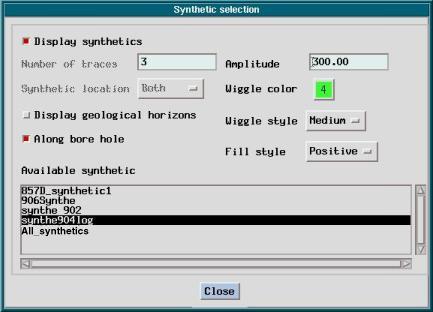
- In the Seis2DV/3DV window, select 'Define/Borehole Appearance/Vertical...' - select the 'Synthetic options...':
You can choose to display the synthetics as one wiggle 'along borehole' - or if you uncheck this option, you can choose to have more than one trace, which can be useful to highlight reflectors.
The synthetics displayed in the list are all the synthetics in the project - so you have to define your names carefully when you save them, to be able to remember the origin and some characteristics of the synthetics.- To display multiple synthetics:
There are two ways to do this:1) When saving the synthetics, give them all the same name (for example here All_synthtetics). When you give the same name to synthteics from two different boreholes, none gets overwritten - but it will appear as just one name in the synthetics selection menu.
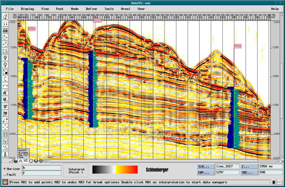
2) Save synthetics in each hole with distinct names (here 906synthe, synthe904log, synthe_902) and define one Borehole Vertical Appearance for each synthetic (in each one of these appearances, you select not to display the logs, and just to display the synthetics of one hole). If you want to also display the logs, make one more vertical appearance with the 'Display synthetics' option off, but where you display the curves (when you post logs on a line., you don't choose the log - it posts the latest available logs from all the site). You have to select this vertical appearance before all the synthetics (like in the figure below, nj_logs before the synthetics), because all appearances are posted on top of each other. If you have chosen to display the logs filled, it is going to hide the synthetics if you don't select it first.
The following figure was made by posting the same borehole set (Leg_150) with all the appearances listed above - one appearance (nj_logs) for all the logs, and one appearance for each synthetic.
It is not possible to send a seismic section or the basemap directly to a printer. To produce a hardcopy, you first have to create a CGM file that you will be able to open in some applications (Canvas with the right plug-in,...) or to send to a plotter through the Larson plotting system (the system currently at Lamont and on the ship - other systems might be available elsewhere). With the Larson system, it is also possible to convert the CGM file into various image format (gif, tiff, jpeg,...) allowing you to open the file in almost all graphic applications.To make a cgm plot of a seismic line:
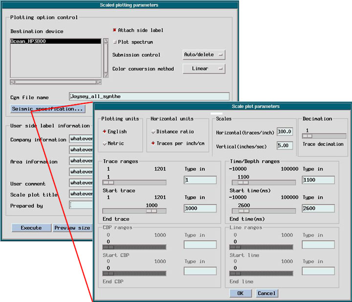
- From the Seis2DV application, File/ Scaled plot... will bring up the 'Scaled plotting parameters; window:
- Give a name to your file
NB: don't try to enter the full path - the file will be in a pre-defined directory:
on treefrog: data/treefrog/gf4/hardcopy_files
(nb: spiff is not active anymore - treefrog is the default lamont host)
on spaceman /data/spaceman/gf2/iesx/scratch
on argo /home/gf4/iesx/scratch
on jason /users/jason/gf6/iesx/scratch.)
NB: don't put .cgm at the end of your name - it will be put automatically
- By default it will print the layout present in the Seis2DV/3DV window. To modify this and have better control of your output, Seismic specification... allows you to change the scales (trace decimation, traces per cm, seconds per cm) and the extents (start and end trace, start and end time).
- The 'absolute' dimensions of the plot are in inches - if later you want to convert your file to another image format with cgm2img, these original dimensions in inches will be the reference values.
- You can write several annotations to your figure in the side label - the lines in the 'User side label information' are here for that. If you don't want the side label, uncheck the 'Attach side label' box.
- Check the size of the output by pressing `Preview Size'. Then `Execute' if the size is OK.If the Larson software is installed on your system:
To send the file to the printer
- Execute 'npsuser' in any unix window to start the Larson interface .
- Select the destination plotter in the right side menu (there should be only one available).
- Press the 'file name' button to popup a window to select your file.
- > a series of printing parameters should appear on the left side when this is done. The default vales are usually fine
- 'View' will give you a preview of your file - it might appear striped if it is a big file, but it should still print ok.
- 'Submit' to sent it to the printer.To convert the cgm file to a standard image format (that you can import into other applications (Illustrator, Photoshop,..)
- Move the cgm file from its location in the scratch directory to a more convenient working directory (your home directory,..)
- The command to convert your cgm file to gif, tif, jpg,... is called cgm2img. The general syntax is:
cgm2img infile -<fmt> [-out <outfile>] [-<bpp>] [-c <type,options>] [-s <image width, height, units>] [-d <dpi>] [-g <gamma>] [-to <trace option>] [-p <cgm picture>] [-r <rotation>]<infile> == CGM input file
-<fmt> == output format: gif, jpg, tif, pdf, cal, pcx, png, ras(Sun raster), bmp(Windows bitmap), xwd
-out <outfile> == image output file
-<bpp> == bits per pixel, 1, 4, 8, 16, or 24
-c <type, option> == compression type, option
-s <width, height, units> == image width, height, in specified units
units is 0, 1, 2 for inches, cm. or pixels
-d <dpi> == dots per inch
-r <rotation> == apply rotation in degrees, 0, 90, 180 or 270If your file name is test_file.cgm, and you want to covert it to a jpeg file named test.jpg with a resolution of 300 dpi the command will be:
cgm2img test_file.cgm -gif -out test.gif -d 300For better control of the aspect of your figure, we recommend you don't use the size (-s) options. By default, it will use the dimensions resulting from your choices of traces/inches and inches/second when creating the cgm file. Giving a high resolution (300 dpi or more) should guarantee the quality of your images. If you still want to use the -s option, be sure to respect your original aspect ratio.
Notes: if the plotting interface (npsuser) or cgm2img do not seem to work, your Larson environment is probably not set up properly: you have to make sure that the following line is in your .cshrc:
setenv LSTHOME /users/jason (at Lamont /users/brg0)
and that $LSTHOME/larson/lstbin (aka /users/jason/larson/lstbin and /users/brg0/larson/lstbin) is in your path.