3.1 The Application Manager
    3.2 Data Management
        3.2.1 The Wells and Borehole Manager
            3.2.1.1 The Well Editor
            3.2.1.2 The Borehole Editor
                Borehole elevation information
                Well Deviation Survey
                Checkshot survey
        3.2.2 The General Data Manager

    3.1 The Application Manager

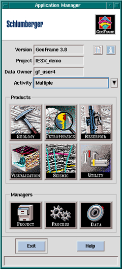
    Open the Application Manager from the Project Manager. Once the Application Manager is open, you can actually close the project manager, which will make one window less...but many more to come.
 

The Application Manager	The Application Manager - activity selection

    The 'Application Manager' allows you to invoke the three 'managers' of a project:

            -The 'Project Manager' already described, but that you might need later, as your project builds up, to change coordinate system, add storage space, or change any parameter described in section 2.

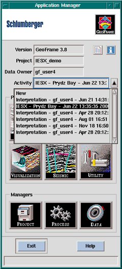
            - The 'Process Manager' which will be described later, in which you build the module (application) chains to process your data. In the 'Activity' menu (which was opened in the right panel by selecting the black arrow) you might want to make a distinction between different activities for one project. One activity could be FMS processing, and the other IESX interpretation. We describe later how to give different names to different activities, but generally you will want to regroup all processing in only one activity. In this case this default activity will appear whenever you click 'Process' to start the process manager. Otherwise, you will have to select first the activity that you want, before starting the 'Process' manager.

            - The 'Data Manager' for all data management tasks (data focus, renaming, deletion, ...)

    In addition, you can open one of the 'Product' catalogs - the 'Seismic' catalog allows a fast access to IESX (see 5.1.1)

    Press the 'Data' icon - the Data Management Catalog will appear; open the 'Data Managers' folder, and double-click both the `General' and the `Wells and Boreholes' data managers.

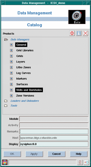
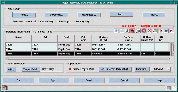
3.2.1 The 'Wells and Boreholes' Data Manager

        This utility allows you to define and edit general parameters for the different levels in the project hierarchy:

Field (Prydz Bay, Nankai trough, ODP Leg 119, ...)
   -> Well (742A,...)
          -> Borehole (Hole 742A,...)

        In ODP operations, there is no actual difference between 'well' and 'borehole': this distinction appears in oil field operations, where multiple deviated 'boreholes' will sprout out of a single 'well' - which is why the 'Surface coordinates' are defined in the 'Well editor' while the deviation and checkshot surveys are defined in the 'borehole editor' (see later sections).

        - First, create a field: press 'Target Field...' and enter a name for your field (e.g. Prydz Bay).
        - Enter the name (e.g. 742A) and UWI (e.g. 742A) of the borehole in the first column.
        - Pressing 'Apply' will fill the well name. The other parameters (coordinates, depths,..) will be edited later in the 'Well Editor' and the 'Borehole Editor'.
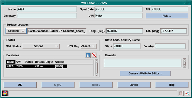
       - Press 'Add...' to add more boreholes.

3.2.1.1 The Well Editor

    - Press the Well Information icon (ringed above) to bring up the Well Editor for the well selected (here 742A).

- Select `Geodetic' as the Surface Location, and enter the Latitudes and Longitudes of the boreholes:

Hole Latitude Longitude

739C -67.2762 75.0818
742A -67.5497 75.4045
1166A -67.696177 74.786925

    - If you select 'Projection' instead of 'Geodetic' in the surface location after entering these values, the values displayed represent the relative coordinates in the projection that you have defined earlier .
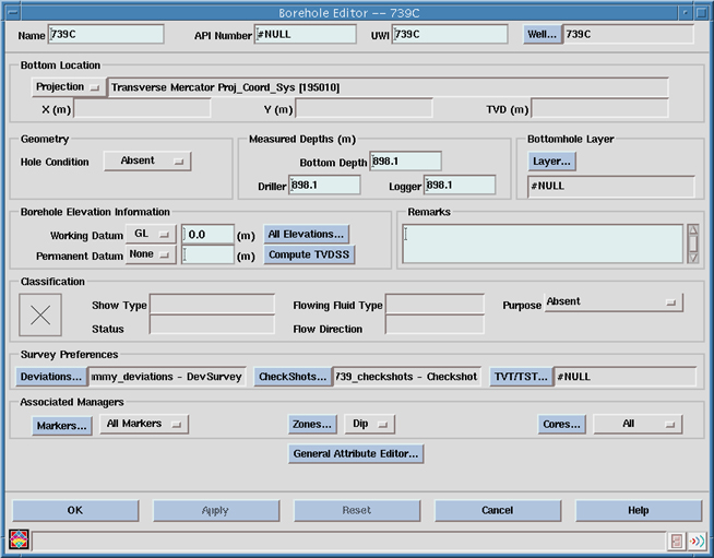
    - 'OK' to get back to the 'Wells and Borehole Manager'

3.2.1.2 The Borehole Editor

    - Double-click on the 'Information' icon in the 'Project Borehole Data Manager' to bring up the Borehole Editor. This menu can also be accessed by double-clicking on the borehole icon in the general data manager, and by double-clicking on the Borehole label on the seismic line or basemap. Its function is mostly to position the borehole and its trajectory in space.
    The 'Borehole Elevation Information' section helps define the reference depth.
    The 'Deviations Survey' defines the trajectory of the borehole. ODP wells are mostly vertical, but GeoFrame does not 'know' it (this is not the case in most oil field operations) so this trajectory has to be defined to be able to display the wells on seismic lines.
    The 'CheckShots survey' defines the time/depth relationship, which is necessary to display logs (measured vs. depth) on a seismic line (which is generally in two way travel time to sea level).

Borehole Elevation information

    - The 'permanent datum' is actually not used at all (it's left over from previous versions) - so it can be left to 'None'
    - The working datum can be understood by default as the 'zero' depth in the logs.
    BOTTOM LINE 1: leave it to 'None' and forget about it. 'Reference depth' issues will be addressed in the checkshot editor.
    BOTTOM LINE 2: use the same depth index for logs and check shot (i.e. both indexed in mbsf or both in mbrf).
    This can be crucial because seismic data will most often be referenced to the sea surface (time=0s), logs are more convenient in meters below seafloor for comparison with cores, and checkshots can be defined either way, with one-way travel time usually from the sea surface. A 'symptom' of bad working datum will be 'squeezed' logs on your seismic lines. If you follow these two rules, there should be no problem. But then again, this is the Realm of GeoFrame...don't take anything for granted.
    See the table at the end of the 'Checkshot' section

Well Deviation Survey

    A deviation survey is required to convert the log data from MD (Measured Depth) to TVD (True Vertical Depth). It's only really critical for deviated boreholes; most ODP holes are sub-vertical, but the software still requires a deviation survey, or the logs in TVD to start with. If the GPIT was run, you can use the DEVI and AZIM logs (you would specify it in the 'Input Data' pull-down menu) - but the simplest way is to 'create' your survey from scratch.

    Note: If you plan to load your logging data from ASCII files you can skip this step by loading your data as functions of TVD instead of 'Measured Depth' (see 'ASCII load') - when the data are referenced to TVD there is no need for the deviation survey.

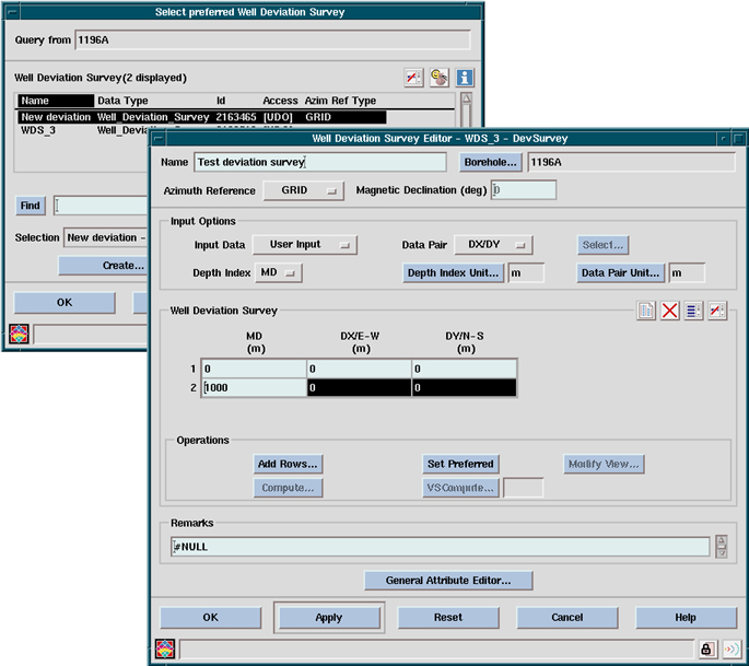
    - Press `Deviations,' then `Create,' to bring up the 'Well Deviation Survey Editor'.

    - Select 'GRID' Azimuth Reference
    - Select 'User Input'  Input Data
    - Select 'DX/DY' data pair
    - Give a name yo your survey (by default it will be called WDS_1,2,...)
    - Give an arbitrary depth (here 1000) in the second row of the table in the MD column
    ->  'Apply'.
                It will warn about a difference between this arbitrary depth and the actual borehole max. depth, which is not a problem
                - Hit 'Compute' - which will pop-up one more window where nothing has to be changed - then 'OK' .

Checkshot survey

   Even if you have no actual VSP or WST checkshot data, you need a checkshot survey to be able to display logs on seismic lines - a sonic log or manual entries can be used for this purpose.

    Note: If you are planning to produce synthetic seismograms, the synthetics will generate the checkshot that you will want to use on your seismic line. The following section is if you want to display your logs on the seismic line without going through the synthetic seismogram generation.

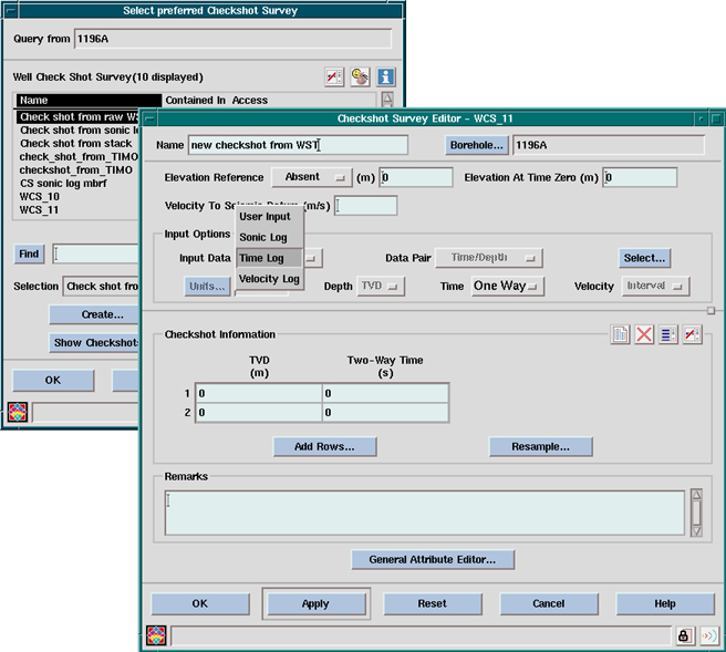
    - Press 'CheckShots...' in the 'Borehole Editor' to open the 'Select preferred checkshot survey' window.

    - If you use checkshot data or an ASCII file with some time/depth values (i.e., two columns, one with depth, the other time), you have to load them first with ASCII load. The checkshot that you have loaded should appear
 

    Entering Data manually

    - Select 'create...' to open the 'Checkshot Survey Editor'.
 
 

 - Give a name to your survey.
 - Select 'User Input' in the 'Input Data' menu.
 - Select 'One Way' or 'Two way' in the 'Time' menu.
 - Add as many rows as necessary with the 'Add rows...' menu.
 - Enter all your values in the table.
 - 'Apply' to validate.
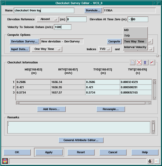
 - 'OK' to proceed.

Using Sonic log data
 - Use the instructions in 'Loading ASCII logs' to load your slowness data (array = DT)
 - Give a name to your survey
 - Select 'Sonic Log' in the input data menu -> most buttons will become dimmed
 - Use 'Select...' to pop-up the 'Select log' window - choose the 'DT' array that you want to use
   -> the following window will appear with only the 'MD' and 'INTV' columns filled.
 - Choose 'TVD' in the 'compute' menu - hit 'compute' to calculate the True Vertical Depth
 - Choose now 'Two Way Time' in the 'compute' menu- then 'compute' - it should now look similar to this window.

    The initial TWT value is based on your initial depth and velocity at this depth (here 0.000324329s = 2*0.2686/1656.34).
    This velocity is usually faster than the sonic velocity in the water column, so you will have to adjust it later with the 'Elevation at Time Zero' and the 'Velocity to Seismic Datum' - once you have displayed the logs on the seismic line you will be able to adjust this.

- 'OK' to proceed

3.2.2. The General Data Manager

    The General Data Manager is one of the most heavily used utilities of GeoFrame. It allows you to keep track of all the data loaded, the modules run, and data generated by any module. It can also be used to edit any kind of parameter, to delete some data items, or to rename items so that they have a 'meaningful' instead of generic name.
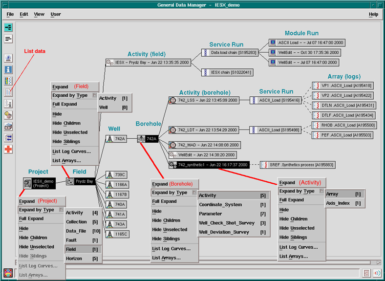
    When you first start it, only the project icon appears (here IESX_demo), in black. You have to 'expand' it to display the subordinate items. In the figure below, some of the items are also in black, which shows that they are 'selected' or 'active'- and that any action that you perform will be applied to these items only. 'Use the 'Control' key to select (activate) multiple items.

- The basic actions are through the 'Edit' menu (which allows you to delete, rename,...) or through the 'View' menu, which is equivalent to clicking the right mouse button (MB3).
- The 'View' options, displayed here for different kinds of items, are basically to 'expand' or to 'hide' items (subordinate = 'children' or on the same level = 'siblings').
- 'Expand by type' allows you to specify what branch(es) to display - the number of available 'types' being different for any kind of item.
- 'Expand' will expand every selected item by one level.
- 'Full Expand' will show every single branch and feature descendant from the selected item(s) - not necessarily recommended at the 'root' of the tree...
- Double clicking on any item will bring up an editor, information, log preview, etc.

When you select 'Expand by Type', only the types existing for the selected item(s) will appear.
In the example below, we have expanded different types of items:
            - The Project was expanded by field -> i.e. Prydz Bay.
            - The field was expanded by well and activity -> the 8 wells in the field and the Activity 'IESX - Prydz Bay' are displayed. This activity corresponds to the one displayed in the 'Application Manager'.
            - The borehole 742A was expanded by activity: the five activities were 3 data loadings, one welledit, and a synthetic seismogram calculation (742_synthetic1).
            - Finally, the synthetic seismogram activity '742_synthetic1' was expanded by arrays, to display the calculated synthetic seismogram.

Notes:

- This is not a 'real' data manager: here we have displayed the menu for each selected item. If these items were actually all selected while pulling down the menu, only one menu would appear, with all the descendants the selected item.
- The number of types and of items in each type will usually increase during the life of a project, so it can be relevant to do some cleaning from time to time.
- The date in the activity names and the numbers in the names of the service run and array are a good way to figure which one is the most recent - the numbers in the array and service run refer to process numbers, which increase with time.
- The example shown here with the synthetic seismogram activity shows how it is possible to locate the results of seismogram processing (or any kind of processing) - and export them.  If you select the array 'SREF. Synthetic process [A195883]' - and hit the icon indicated here with 'List data', you will open the 'data viewer', that allows you to display the values on the screen or to write an ASCII file.

    The other way to access your logs or arrays is to select any well or borehole in the General Data Manager and then select the 'List Arrays...' option in the menu (see below, where we listed arrays for Hole 742A). This will open the 'Array list' window, with all logs and arrays associated with the selected borehole:

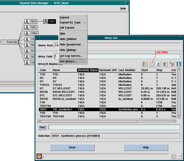
    In the example shown here, the logs available for Hole 742A include density (RHOB), travel time (DT), TVD (True Vertical Depth), TWOTIM (two way travel time) and SREF (the synthetic seismogram). 'DX', 'DY' and 'TVD' were produce by the creation of the Deviation Survey.
    The 'Last Modifier' field indicates what module or activity (if any) was used to produce it. In particular, the 'WELLEDIT' modifier indicated logs that were edited with the WellEdit module, which is used to edit logs in GeoFrame (cleaning, despiking, smoothing, depth-shifting, merging, extrapolation to seafloor,...). For a typical IESX-related project, the logs at the beginning of the project are DT and RHOB.
    To export any of these logs to an ASCII file: select the log(s) in the Array list (use the Control' key to select multiple logs) - and then hit the Icon indicated by 'List data'.