4.1 The Process Manager
    4.2 Loading Log Data
        4.2.1 Loading DLIS data
        4.2.2 Loading ASCII data
        4.2.3 Loading ASCII checkshots
    4.3 Editing log data using WellEdit

    4.1 The Process Manager

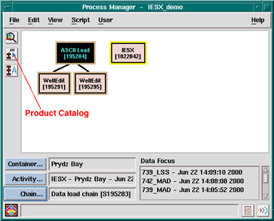
    The Process Manager allows you to select and run `modules' (=applications), which are associated in processing 'chains'.
    The example below shows the same process manager, with two chains - on the left the 'Data Load Chain' is selected - on the right the 'IESX Chain'.  The 'container' is the same (Prydz Bay, the field), the activity is the same ('IESX - Prydz Bay', see in the 'General Data Manager' and in the 'Application Manager'). In the General Data Manager the two chains appear as 'Service Run' for the activity. A chain is selected whenever one of it's modules is selected (black). The default names of the chains are rather uninformative (aka. "geoframe interpretation"), so if you use multiple activities and/or multiple chains, it is better to rename them, by selecting the 'Chain...' button.

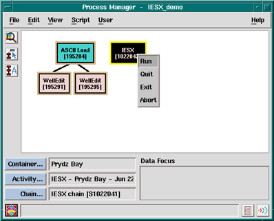
    To Run a module - select it - press the right mouse button (MB3) to make the menu appear (see right process manager panel below)- select 'Run'
    To abort a module - it is sometimes necessary to 'abort' a module (IESX, Borview,... ) when it has been frozen for some time and it is clear that nothing is happening.
        To do so - MB3 -> 'Abort'. The edge of the module will turn red.
        This is equivalent to 'killing' the process with its ID number in a unix terminal - which might be necessary if the process manager itself is frozen.
 

To add a module:

    To start a new chain: deselect all modules (click in the white space) - and open the 'Product Catalog' (shown below) by clicking the middle icon indicated on the left.

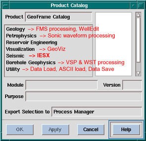
    To add a module to a chain: select the existing module where the new module should be connected - and start the product catalog. The new module will appear under the previous one.

    4.2. Loading Log Data

    The minimum log data that is required for running the Synthetic Seismogram application is sonic travel time data. Other data to load, if you have them, are the density log, and the core moisture and density measurements.

    ODP core data are available from: http://www-odp.tamu.edu/database
    Log data from: http://www.ldeo.columbia.edu/BRG/ODP/DATABASE/DATA/search.html

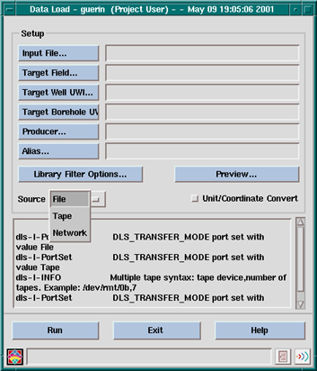
4.2.1 Loading DLIS data

   If you have DLIS data, use the Data Load module (in the 'Utility' section of the 'Product Catalog')

    - Select the 'Source' - File if it's on a hard drive or a CD-ROM - 'Tape' if it's on a DAT, an hexabyte, or any other magnetic device. In the later case, the device has to allocated, and the name should be /dev/rmt/0lbn (see previous discussion for project backup/restore).
    - The field and borehole names should be in the header file - in this case, these parameters will be filled automatically - but it is possible that the Schlumberger Engineer did not put the correct field and/or borehole name - or that the names he gave at acquisition time are different from the names you created in your project, so it is recommended that you fill these parameters (Target field..., Target well..., Target borehole... ) to make sure the data get affected to the right hole.
    - 'Preview...' allows you to control what logical files to load.
    - 'Run' to actually load the data - this can take a while.
    - 'Exit' once it's done.
    - Warning - when you exit, a popup window asks if you want to delete what you just loaded - select 'cancel' to make sure this does not happen.
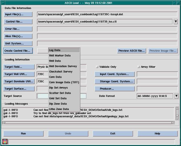
    - Proceed to edit the data.

4.2.2 Loading ASCII data

    To import ASCII data (either logs, core data or check shot/reflectors depths) use ASCII Load (in the 'Utility' section of the 'Product Catalog').

- 'Input files(s)...' pops up a menu to select your ASCII file(s).
- 'Control file...' has to be defined the first time around - it will keep track of your loading parameters.
- Error and Alias files have not much relevance.
- in the 'Loading Information' area, set the 'Target Field..', 'Target Well...' and 'Target Borehole ...' to the correct values so that the data get affected to the correct hole.
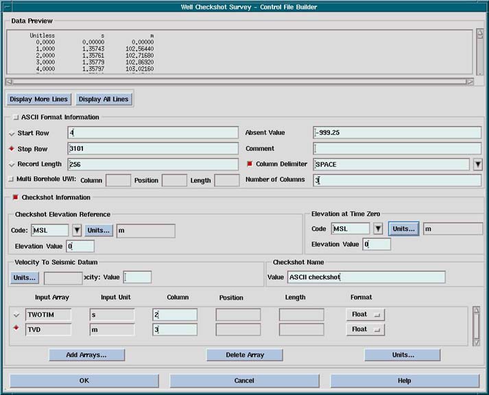
- Select 'Create Control File...' to open the 'Control File Builder' (below), where you will enter the parameters necessary to read the data. Because it is pretty flexible on the original format of the ASCII data, you will have to enter quite a few parameters.

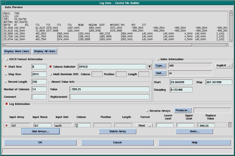
- The upper part of this window gives a preview of the ASCII file, with likely some header lines
- The 'ASCII format information' area is used to describe the input file.
- The 'Index Information' area is used to define what kind of indexing parameter is used (aka depth, TVD, time...) - and whether the indexing is implicit (given an initial and a final value and an increment) - or explicit - where you have to specify the column where the index will be read.
        For logs, use 'Implicit' - with a sampling interval of 0.1524 - for some reason, if you use 'explicit' instead, you won't be able to calculate synthetic seismograms
        For core and WST (check shot) data, select 'Explicit' - and enter the column with the index value.
- The 'Log Information' area is used to define the data to be loaded.

To fill it:
       If the 'Start Row' button is selected (red), click on the first line of good data in the 'Data Preview' window to enter automatically it's number.
       If  you are loading implicit log data, enter the value (depth) of this first row in the 'Start' section of the 'Index Formation' area and the sampling rate (0.1524).
       Check the 'Stop Row' button .
       Click on 'Display All lines' to get to the end of the file in the Preview.
       Click on the last line of good data in the 'Data Preview' window to enter automatically it's number in 'Last Row' .
       Enter the value (depth) of this last row in the 'Stop' section of the 'Index Formation' area.
       Enter the 'Number of Columns' present in the ASCII files - you should not worry about the 'Record Length'
       Select the nature of the Column Delimiter (space, tabs,...)
       In the 'Index Information' area: 'Type...' will popup the possible types of index. MD (measure Depth) or TVD (true vertical depth) for most data. If you use TVD, you should not need any deviation survey.
       'Unit...' should be m (meter) by default.
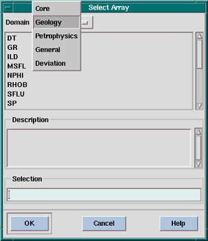
       In the 'Log Information' area - click 'Add Array...' to open the 'select array' menu:

    Most available log data are in the 'Geology' domain (DT = slowness, RHOB = density, GR = Gamma Ray,...)
    Make sure you use array names that can be identified by IESX for synthetic seismogram processing. These arrays can be only DT and RHOB (not DTLN, HROB,... even though they represent the same type of data)
    If you are loading check shot, the proper array name is '1WAY' in the 'General' domain.
    -> OK to close this menu
    Back to the 'Control file builder' enter the column number of the data in the ASCII file (2 in this example) in the 'Column' field of the 'Log Information' area.
    'OK' to close the 'Control file Builder'
    -> back to the ASCII Load window, 'Run' to load the data.
    Repeat all the steps above for all the logs you want to enter. It keep tracks of all parameters, so you will only have to change some of the parameters for each log (the file name, the column number, the type, the start and stop,...

4.2.3 Loading ASCII checkshots

    Checkshot data in ASCII form should be organized in columns with one column for the depth of the checkshot (or marker) and one column with the travel time (either one-way or two-way).
    To avoid the headache of what reference to use and to define (which, whatever you read is never totally clear), things should run smoothly if your checkshot includes points at the top and at the bottom of your logged intervals.

    To load the data:
    - Select 'Checkshot Survey' in the 'Create Control File...' pull-down menu in the 'ASCII Load' window.
    - 'Create Control File...' will pop up this window:

- The parameters in the 'ASCII Format Information' are similar to standard ASCII load.
- Even if you put '0' as elevation value for time zero and for the checkshot elevation reference, you have to pick a unit in the two 'Checkshot Information' boxes.
- If your checkshot includes data points at the top and at the bottom of your logs, just use 0 as the elevation values
- Add two arrays - one TVD - the depth of the checkshots - and one TWOTIM or 1WAY (depending on the type of checkshot you have).
- 'OK' to get back to the 'ASCII Load' window, then 'Run'.

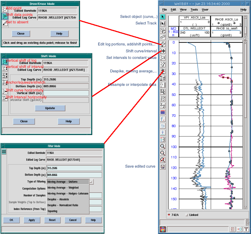
    The log data must undergo a certain amount of editing before they can be used in the IESX Synthetics application. In particular, it can be useful to extend the logs to the seafloor to simulate an approximate location for the seafloor reflection.
    In the Hole 742A example data shown here, the log density had some bad values due to hole washouts; core-based density measurements, interpolated onto even spacing, were used instead.
    Other typical tools include filtering, despiking or smoothing data (see filter mode panel in figure), shifting data vertically (in depth) or horizontally (the data values), and adding or erasing points (draw/erase mode) - this latest tool is the one used to extrapolate data to seafloor.

    To extrapolate to seafloor (this is in no way necessary - it can be convenient to have a reflection at the seafloor, but synthetics can be made without doing this extrapolation):
            - Select the curve you want to edit with the 'Select Object' tool.
            - Select the Draw/Erase mode (5th button from top, with the crayons).
            - Select the first button in the 'Draw / Erase Mode' window.
            - Click on the seafloor with the left mouse button (MB1) (depth = 0 mbsf) at reasonable values for the curve you are editing (200 ms/ft for slowness, ~1.3 g/cc for density). You can also add other intermediate points. Click MB3 (right mouse button) to finish - the edited curve will appear in red, connecting automatically to you shallowest data.
            - 'Close' the 'Draw/Erase' window.
            - Use other tools if necessary - all changes that you make will apply to the curve that you selected in the first place until you save it.
            - To save it - use either the lowest 'floppy' button on the left or 'File/Output....'
            - When you save, put a name in the 'modifier' that will allow you to identify the new curve later - this modifier will be the suffix of your file name.
Note: the original log curve is actually not affected - you are creating a new curve with the same code.