Sonic Digital Tool (SDT*)
Description
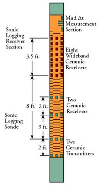 In fast formations, where shear velocity is faster than the velocity of the drilling fluid, the SDT obtained direct measurements for shear, compressional, and Stoneley wave values. In a slow formation, the SDT obtained real-time measurements of compressional, Stonily, and mud wave velocities. Shear wave values could then be derived from these velocities. This multireceiver sonic tool, with its linear array of eight receivers, provided more spatial samples of the propagating wavefield for full waveform analysis than the standard two-receiver tools. This arrangement allowed measurements of wave components propagating deeper into the formation past the altered zone.
The depth of investigation cannot be easily quantified; it depended on the spacing of the detectors and on the petrophysical characteristics of the rock, such as rock type, porosity (granular, vacuolar, fracture porosity), and alteration. For source-detector spacings of 3-5 ft, 8-10 ft, and 10-12 ft the depth of investigation ranged from 2 in to 10 in (altered/invaded and undisturbed formation, respectively), 5 in to 25 in, and 5 in to 30 in. The vertical resolution was 2 ft (61 cm).
Until 1999, the SDT was used extensively in combination with the Formation MicroScanner (FMS) during the Ocean Drilling Program. It was run in one of two modes: depth-derived borehole compensated (DDBHC) or linear array. In DDBHC mode, the SDT was capable of operating in both short- and long-spaced modes, and the modes coiuld be run simultaneously when compressional slowness measurements were needed over a wide range of spacings. In linear array mode, the SDT acquired compressional, shear and Stonely waveforms.
Applications
Porosity and “pseudodensity” log. The sonic transit time can be used to compute porosity by using the appropriate transform and to estimate fracture porosity in carbonate rocks. In addition,it can be used to compute a “pseudodensity” log over sections where this log has not been recorded or the response was not satisfactory.
Seismic impedance. The product of compressional velocity and density is useful in computing synthetic seismograms for time-depth ties of seismic reflectors.
Sonic waveforms analysis. If a refracted shear arrival is present, its velocity can be computed from the full waveforms, and the frequency content and energy of both compressional and shear arrivals can also be determined.
Fracture porosity. Variations in energy and frequency content are indicative of changes in fracture density, porosity, and in the material filling the pores. In some cases compressional-wave attenuation can also be computed from the full waveforms.
Environmental Effects
One common problem was cycle skipping: a low signal level, such as that occurring in large holes and soft formations, could cause the far detectors to trigger on the second or later
arrivals, causing the recorded dt to be too high. This problem could also be related to the presence of fractures or gas.
Transit time stretching appeared when the detection at the further detector occurred later because of a weak signal. Finally, noise peaks were caused by triggering of detectors by mechanically induced noise, which caused the dt to be too low.
Log Presentation
DT/DTLN and DTL/DTLF are delay times in microseconds per foot for the near and far receiver pairs, respectively. In very slow formations DTL/DTLF provide the more reliable measurement as the refracted wave is not seen at the near receivers. The acoustic data is usually presented as compressional and, where available, shear velocity in km/s.
Output of acoustic data in shallow hol
Output of acoustic data in deep water
| Temperature rating: | 350° F (175° C) |
| Pressure rating: | 20 kpsi (138 MPa) |
| Diameter: | 3.625 in (9.21 cm) |
| Length: | 37.9 ft (11.6 m) |
| Acoustic bandwidth: | 5 kHz to 18 kHz |
| Waveform duration: | 5 ms nominally, 10 ms maximum |
| Sampling interval: | 6 in (15.24 cm) |
| Maximum logging speed: | 1700 ft/hr (518.16 m/hr) for eight receiver array |
| DT: | Acoustic slowness, DDBHC Mode (3-5-5-7 ft), Short Spacing (µsec/ft) |
| TT1: | DDBHC Short-Spaced Mode, Transit Time 1 (5 ft spacing; µsec) |
| TT2: | DDBHC Short-Spaced Mode, Transit Time 2 (3 ft spacing; µsec) |
| TT3: | DDBHC Short-Spaced Mode, Transit Time 2 (3 ft spacing; µsec) |
| TT4: | DDBHC Short-Spaced Mode, Transit Time 4 (5 ft spacing; µsec) |
| DTL: | Acoustic slowness, DDBHC mode (3-5-5-7 ft), Long Spacing (µsec/ft) |
| ITT | Integrated Transit Time (sec) |
| DTLF: | Acoustic slowness, DDBHC Mode (8-10-10-12 ft), Long Spacing Far (µsec/ft) |
| DTLN: | Acoustic slowness, DDBHC mode (8-10-10-12 ft), Long Spacing Near (µsec/ft) |
| LTT1: | DDBHC Long-Spaced Mode, Transit Time 2 (10 ft spacing; µsec) |
| LTT2: | DDBHC Long-Spaced Mode, Transit Time 2 (8 ft spacing; µsec) |
| LTT3: | DDBHC Long-Spaced Mode, Transit Time 4 (12 ft spacing; µsec) |
| LTT4: | DDBHC Long-Spaced Mode, Transit Time 4 (10 ft spacing; µsec) |
| TT1: | DDBHC Short-Spaced Mode, Transit Time 1 (5 ft spacing; µsec) |
| TT2: | DDBHC Short-Spaced Mode, Transit Time 2 (3 ft spacing; µsec) |
| TT3: | DDBHC Short-Spaced Mode, Transit Time 3 (7 ft spacing; µsec) |
| TT4: | DDBHC Short-Spaced Mode, Transit Time 4 (5 ft spacing; µsec) |
| ITT | Integrated Transit Time (sec) |
| DTCO: | Compressional Delay Time (µsec/ft) |
| DTSM: | Shear Delay Time (µsec/ft) |
| DTST: | Stoneley Delay Time (µsec/ft) |
| ITT: | Integrated Transit Time (sec) |
* ®trademark of Schlumberger