Category Archives: Technology

Compensated Neutron Dual Porosity Tool (CNT-G*)

Compensated Neutron Dual Porosity Tool (CNT-G*)

Description
The CNT-G tool employed a chemical source (Am-Be) to bombard the borehole and the formation with fast neutrons (4.5 MeV) and two pairs of sensors to detect the number of neutrons (count rates) in the epithermal (100 eV – 0.1 eV) and thermal energy range (<0.025 eV). In the scattering process the neutrons interacted elastically with the atoms in the formation, were slowed down, and lost part of their kinetic energy with each collision; upon reaching the thermal energy level, they were absorbed by the surrounding nuclei. The amount of energy lost by the neutrons depended on the relative mass of the nuclei with which they interacted Because the greatest energy loss occurs during the collision with hydrogen atoms – which have a mass almost equal to that of neutrons – the slowing down and capture processes were mainly controlled by the hydrogen concentration in the formation. By taking the ratio of count rates at each pair of detector, a measurement of the porosity of the formation — compensated for the borehole parameters — was provided.
The response at the thermal detectors could be greatly affected by elements with a large thermal neutron capture cross section, such as chlorine, boron, gadolinium, and samarium; these are usually present in very small quantities in the borehole fluid or in clay or alteration minerals, yet they can cause the porosity of the formation to be overestimated. The epithermal detectors, instead, were less sensitive to these neutron absorbers and provided a more reliable measurement of the true porosity of the formation over clay-rich intervals. Because the epithermal neutron count rate is about one order of magnitude less than that for the thermal neutrons, the detectors were placed closer to the source in order to improve statistical variations.
The CNT-G was deployed extensively during the Ocean Drilling Program.


Applications

Porosity
In reservoir engineering its importance is quite evident; in the study of the volcanic rocks that make up the upper oceanic crust, a good in-situ porosity measurement is most important to the correct understanding of the crustal structure: first, because it samples both the small-scale (microcrack, vesicle) porosity seen in the cores and the large-scale fractures not sampled by drilling; and second, because other properties such as density, seismic velocity, and permeability, depend strictly on porosity variations and on the geometry of the pore space. In the presence of clays or hydrous alteration minerals a correction is required to account for the presence of bound water.

Lithology
Because the hydrogen measured by the tool is present not only as free water but as bound water in clay minerals, the porosity curve, often combined with the density log, can be used to detect shaly intervals or minerals such as gypsum, which has a high hydrogen index due to its water crystallization. Conversely, the neutron curve can be used to identify anhydrite and salt layers (which are both characterized by low neutron readings and by high and low bulk density readings, respectively).


Environmental Effects
Eccentralization of the tool by a bow spring could be very helpful in obtaining reliable porosity measurements. The lack of contact of the tool with the borehole wall during the recording results in the attenuation of the formation signal by the borehole fluid and, in turn, the likely overestimation of the true porosity of the formation. In the majority of ODP holes, however, the CNT-G was run without an eccentralizer.
Hole size also affects the neutron log response: the formation signal, particularly for the epithermal count rates, tends to be masked by the borehole signal with increasing hole size.
In liquid-filled holes the influence of the borehole fluid depends on its salinity – chlorine is a strong absorber – and density: the addition of weighting additives such as barite will yield a lower porosity reading.
In the Ocean Drilling Program, the neutron tool was sometimes recorded through the drilling pipe and the bottom hole assembly. Because iron is a strong neutron absorber, the effect was an increased porosity reading, depending on the thickness of the pipes.


Log Presentation
The CNT-G provided an epithermal (ENPH) and thermal neutron porosity (NPHI) measurement. The porosity curves were presented either in decimal units or in percents along with the bulk density.


Tool Specifications
Temperature rating: 400° F (200° C)
Pressure rating: 20 kpsi (138 MPa)
Diameter rating: 3.375 in (8.6 cm; without bow spring eccentralizer)
Length: 7.25 ft (2.21 m)
Weight: 120 lbs (54 kg)
Sampling interval: 6 in (15.24 cm)


Measurement Specifications
Vertical resolution: 12 in (30.48 cm)
Depth of investigation: ~ 9 in (22.9 cm)
Accuracy:
0-20 pu: ±1 pu
30 pu: ±2 pu
45 pu: ±6 pu


Main Outputs
ENPH: Epithermal Neutron Porosity (pu)
TNPH (or NPHI): Thermal Neutron Porosity (pu)
CFEC: Corrected Far Epithermal Counts (cps)
CFTC: Corrected Far Thermal Counts (cps)
CNEC: Corrected Near Epithermal Counts (cps)
CNTC: Corrected Near Thermal Counts (cps)
ENRA: Epithermal Neutron Ratio
TNRA: Thermal Neutron Ratio


Deployment Notes The CNT-G was typically run in combination with the density and gamma ray tools.


*®trademark of Schlumberger

Compensated Neutron Log (CNL*)

Compensated Neutron Log (CNL*)

Description
The compensated neutron log tool (CNL) contained a 16-curie Am/Be radioactive source that bombarded the formation with fast neutrons and two detectors at different spacings from the source. The neutrons were slowed down through elastic collision with the formation nucleii and then captured, primarily by hydrogen atoms in the formation. The slowed neutrons deflected back to the tool were counted by detectors. The tool responded primarily to the hydrogen content of the formation because hydrogen has a mass close to that of the neutrons and thus is most efficient in the slowing process.
The measurements (ratios of far to near detector counts) were transformed to porosity units on the basis of laboratory calibrations. The 16-curie source produced neutrons at four times the rate of a standard nuclear source, greatly reducing statistical variation. The use of longer source-to-detector spacings increased the depth of the investigation.
The CNL was used during the Deep Sea Drilling Project.


Applications

Porosity
In reservoir engineering its importance is quite evident; in the study of the volcanic rocks that make up the upper oceanic crust, a good in-situ porosity measurement is most important to the correct understanding of the crustal structure: first, because it samples both the small-scale (microcrack, vesicle) porosity seen in the cores and the large-scale fractures not sampled by drilling; and second, because other properties such as density, seismic velocity, and permeability, depend strictly on porosity variations and on the geometry of the pore space. In the presence of clays or hydrous alteration minerals a correction is required to account for the presence of bound water.

Lithology
Because the hydrogen measured by the tool is present not only as free water but as bound water in clay minerals, the porosity curve, often combined with the density log, can be used to detect shaly intervals or minerals such as gypsum, which has a high hydrogen index due to its water crystallization. Conversely, the neutron curve can be used to identify anhydrite and salt layers (which are both characterized by low neutron readings and by high and low bulk density readings, respectively).


Environmental Effects
The tool was designed to minimize the effect of hole size. When run in combination with the FDC (formation Density Compensated Tool), the caliper measurement was used to apply an automatic correction for hole diameter. Other factors that might affect the porosity reading were temperature, salinity, lack of eccentralization (standoff) and type of drilling fluid.


Log Presentation
The CNL was recorded in linear porosity units (or %) for a particular matrix lithology (limestone, sandstone, dolomite, usually limestone). When a CNL was run in combination with another porosity log, both curves were recorded on the same porosity scale. This overlay-type presentation permitted visual qualitative interpretation of porosity and lithology or the presence of gas.


Main Outputs
NPHI: Neutron porosity (%)
NCNL: Near detector counts (cps)
FCNL: Far detector counts (cps)


Tool Specifications
Diameter: 3.375 in (8.6 cm)
Sampling interval: 6 in (15.24 cm)


Deployment Notes
The CNL was usually run in combination with the FDC or LDT tools.


*®trademark of Schlumberger

Azimuthal Resistivity Imager (ARI*)

Azimuthal Resistivity Imager (ARI*)

Description
ari_small The Azimuthal Resistivity Imager (ARI) was a laterolog tool that made deep measurements and azimuthal resistivity images around the borehole. At the time it helped analyze features and details that escaped conventional resistivity measurements: thin beds (down to 8 in, 20 cm), borehole formation heterogeneity, formation dip, resistivity in dipping beds, and fracture position and orientation. The ARI produced images similar to the FMS with coarser vertical resolution, but complete azimuthal coverage. Whereas FMS electrodes are pad-mounted and in contact with the borehole surface, the ARI provided a remote image of the formation in a similar way to that of the BHTV.
The ARI electrode array operated simultaneously at two frequencies: 35 Hz for the deep readings and 280 Hz for shallow readings. It focused currents that flowed from the 12 electrodes to the grounded logging cable. The sum of these 12 readings produced a high-resolution measurement equivalent to a single laterolog electrode of the same height. To correct for tool eccentralization and variations in borehole shape, a shallow auxiliary measurement of electrical resistivities was performed at a much higher frequency of 71 kHz. This measurement responds primarily to the volume of borehole fluid affecting each electrode. If the borehole fluid resistivity is independently measured, then borehole size and shape can be deduced from the auxiliary array measurements. While the vertical resolution of the standard laterolog readings at the time was about 0.60 m, the high-resolution array could reduce this by up to a factor of 6, depending on the formation resistivity.
The ARI was deployed during ODP Leg 174B (Mid-Atlantic Ridge).


Applications

Thin beds: The deep, high resolution measurements (vertical resolution of < 1 ft) can be used in the quantitative evaluation of laminated forms.

Fractured formations: The ARI response is affected by the presence of fractures filled with conductive fluids. Though ARI images do not have the same definition and resolution of FMS images, open fractures  are clearly visible; some vertical fractures and cracks that may have been induced by drilling, however, may not be clearly visible on the ARI, because they are too shallow to be detected by the deeper reading ARI.

Dips: The formation dip can be derived from the ARI images, though the estimate does not have the accuracy of that derived from an FMS image. ARI images are useful to detect uncomformities and faults, and to confirm expected features.

Borehole profile: The 12 auxiliary-mode azimuthal borehole curves show tool eccentering and borehole irregularities, such as ovality. The ARI electrical calipers are more sensitive to borehole variations than the FMS orthogonal calipers.


Environmental Effects
The electrical standoff measurements can be used to correct the azimuthal resistivities for tool eccentering and variations in borehole shape and size.


Log Presentation
The LLD and LLS measurements are usually displayed on a resistivity logarithmic scale, along with the gamma ray log.
ariplot
Tool Specifications
Temperature rating: 350° F (175° C)
Pressure rating: 20 kpsi (13.8 MPa)
Diameter: 3.625 in (9.21 cm)
Length: 33.3 in (10.1 cm)
Weight: 578 lbs (262.4 kg)
Sampling interval: 6 in (15.24 cm)
Max. logging speed: 1,800 ft/hr (550 m/hr)


Measurement Specifications
Measurement range: 0.2 to 100,000 Ω.m
Vertical resolution: Less than 1 ft (30.24 cm)


Main Outputs
LLD: Deep laterolog (Ω.m)
LLS: Deep laterolog (Ω.m)


Deployment Notes
The ARI was used in combination with density, porosity and gamma ray tools. In order to properly orient the images, however, the ARI had to be used with the GPIT, as is the case for the FMS tool. Repeat passes of the ARI were useful to obtain consistent azimuth measurement.


* ®trademark of Schlumberger

Dipole Sonic Imager supplementary information

Explanation of Acoustic Wave Propagation Monopole compressional and shear Compressional and shear waves (sometimes referred to as p- and s-waves) are excited in the formation, along with various modes in the borehole, by a monopole source operating at high frequencies (typically 10-20 kHz). They propagate as body waves in the formation and along the borehole. As they do so, they leak energy (refract) back into the borehole, creating headwaves in the borehole fluid. Compressional waves propagate along the borehole in the direction of the borehole axis with minute vibrations (or displacements) of the formation in the same direction. Shear waves propagate in the direction of the borehole axis with minute radial vibrations of the formation. Monopole shear waves have a lower velocity (higher t), generally a larger amplitude, and a slightly lower frequency than the compressional waves. Shear waves have a larger refraction angle than the compressional waves. The mud speed is usually nearly constant, so that the refraction angle depends on the phase velocity of the body wave in the formation. As the shear t becomes large (soft formations), less shear energy is refracted back into the hole. If the shear t surpasses the mud slowness (typically 190 sec/ft), none of the shear waves will be detected by the receivers. Monopole Stoneley At low frequencies, perhaps a few kHz, where typical wavelengths in the mud are greater than the borehole size, monopole signals are dominated by the Stoneley wave, a dispersive mode of the borehole. Stoneley waves are guided waves associated with the solid-fluid boundary at the borehole wall, and their amplitude decays exponentially away from the boundary in both the fluid and formation. At extremely low frequencies, the slowness of this mode approaches that of the tube wave, while at higher frequencies, it approaches that of the Scholte (planar interface) wave. It is most easily excited using a low-frequency monopole source. For all frequencies, the Stoneley slowness is determined predominantly by the mud and to a lesser extent by the formation compressional and shear slownesses, formation permeability, and other variables. Dipole shear In a dipole shear sonic tool, a directional (dipole) source and directional receivers are employed. The source is operated at low frequencies, usually below 4 kHz. Compressional and shear waves are excited along with a dispersive flexural mode of the borehole. The slowness of this mode has the same high-frequency limit as the Stoneley wave, but at low frequencies it approaches the formation shear slowness rather than the tube wave slowness. The amplitudes of both the flexural and the shear wave are peaked in frequency, the flexural generally peaking higher. They fall off very rapidly toward low frequencies and more gradually toward high frequencies. The flexural mode dominates the response down to very low frequencies where the shear wavelength is several times the borehole diameter. At such low frequencies, the direct shear wave is the only appreciable feature on the waveform. However, the amplitude of the waves at these frequencies (below 1 kHz for a typical slow formation) is very low and noise is likely to be a problem. A practical frequency range is 1-4 kHz. In this range, the flexural mode dominates the signals, but travels at nearly the shear slowness. A continuous shear log then is obtained by measuring the flexural slowness at as low a frequency as is practical and applying a small correction. In very fast formations, the dipole compressional signal is usually very weak and may not be visible. The flexural mode is very dispersive in fast formations, there being as much as a factor of two difference in slowness between low frequencies (shear slowness) and high frequencies (Scholte slowness, approximately the mud slowness). The flexural arrival is therefore quite long in duration and spreads rapidly as the transmitter receiver spacing is increased. Low-frequency components traveling near the shear slowness become well separated from the slower higher frequency components. Often the (nondispersive) shear headwave is detectable in fast formations. In slow formations, the flexural mode is again dispersive, but to a much lesser extent. Typically, the ratio between the high- and low-frequency limiting values of the flexural slownesses is about 1.2 or less. The flexural arrival is shorter in time duration and the spectral content is concentrated at lower frequencies. As in the figure, a higher frequency compressional arrival is often visible in slow formations, and in large boreholes and very slow formations can become the largest amplitude event. A distinct shear headwave arrival cannot be detected in slow formations.
Slowness Time Coherence (STC) Analysis Acquisition Software Slowness-Time Coherence examines each waveform set for coherent arrivals across the array. It does this by stepping a time window of fixed duration through a range of times across the waveforms and a range of slowness across the array. For each time and slowness step, the waveforms within the window are added or stacked and the corresponding stacked or coherent energy is computed. When the window moveout or slowness aligns with a particular component moveout across the array, the waveforms within the window add in phase, maximizing the coherent energy. Coherent arrivals are thus identified by maxima in the coherent energy. The STC module is used to find and extract slowness (Dt) and other information about various coherent arrivals in the sonic waveforms. Then the STC computation performs a sequence of operations on a set of waveforms aimed at identifying coherent arrivals in the set and extracting their slownesses. The following steps taken are: Waveform filtering, Waveform stacking, Peak searching, and Labeling. An additional step is needed to identify and separate the desired arrivals (flexural, compressional, shear, or Stoneley) from any others. This is done by the labeling algorithm part of the STC computation. The slowness, arrival time, and coherence of each arrival are examined and compared with the propagation characteristics expected of the compressional, shear or Stoneley waves for the given physical conditions. Classifying the arrivals in this manner gives a continuous log of wave-component slowness versus depth. STC processing of high-frequency monopole waveforms generally results in compressional and shear slowness estimates in fast formations. Narrow band filtering is applied to low-frequency monopole (Stoneley) waveforms, since this mode is dispersive and we want to estimate slowness within a consistent band of frequencies. In slow formations, no shear slowness estimate is available from monopole waveforms. Dipole labeling bias correction In STC processing of dipole waveforms, a coherence peak corresponding to the dispersive flexural mode occurs at a slowness near that of the frequency of peak excitation after filtering. The estimate is therefore biased slower than the true shear, and must be corrected. The bias depends on the time signature of the source excitation, the filter characteristics, the borehole size and shear slowness. In slow formations, the correction is less than 10%, and usually much less. In fast formations, where the dispersion of the flexural mode is greater, a large correction is required only in large (>17 in.) boreholes. In a fast formation with a moderate hole size (<12 in.), very little or no bias is found. Depth-derived borehole compensation One way to obtain borehole compensation is to derive slowness (delta t) measurements from both upward and downward propagating waves. The effects of borehole size changes tend to have an opposite effect on the slownesses derived from each. The standard BHC tool accomplishes this by having a transmitter above and below the receivers. The Long Spaced Sonic (LSS) tool, though, simulates this with depth-derived borehole compensation. The DSI-2 employs the same depth-derived technique. Instead of having transmitters above and below the array, it constructs a pseudo-transmitter array from several tool positions as it moves up the hole. The pseudo-transmitter array looks like an array of transmitters with one receiver above. This approximates a single transmitter on top with a receiver array below.
* ®trademark of Schlumberger

Applications of gamma ray logs

Depth correlations and core-log integration

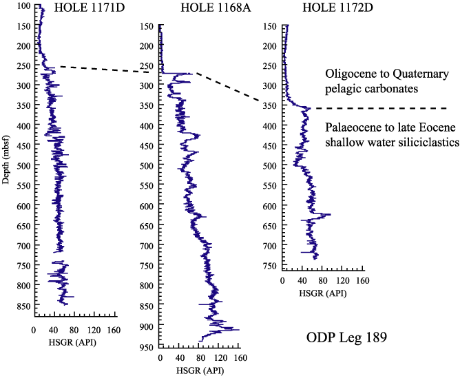
Total gamma-ray log curves, which are acquired with every toolstring combination, are normally used to depth match all of the logsobtained in any one hole. The HSGR log from the Triple Combo is used as the base curve, and the SGR logs from all the other toolstringsare interactively matched to it. The depth shift applied to each SGR curve is propagated to all other logs acquired by that toolstring.Gamma ray data can also be used for core-log integration, by correlating the natural gamma results from the whole core multisensor track (WC-MST) with the HSGR and SGR curves. Furthermore, because the gamma ray log responds principally to fluctuations in the formation’s mineralogy, rather than physical properties such as lithification, it is particularly useful for making regional, inter-hole comparisons between major lithostratigraphic units (Figure 1).

fig1

Figure 1. Regional Correlation of major lithostratiraphic units, using total gamma ray data from ODP Leg 189.

    Identification of lithology, facies and depositional environment

Naturally radioactive elements tend to have a far greater concentration in shales than in other sedimentary lithologies, and therefore the total gamma-ray log and, in particular, the corrected gamma-ray log (HCGR and CGR) and the Th log are frequently used to derive a “shale volume” (see Ellis 1987 and Rider 1996). In addition, the shape of the gamma log curve may be used to reconstruct downhole fluctuations in grain size, and infer changes in sedimentary facies: the standard approach is to interpret bell shaped gamma curves as a fining-upwards sequence and funnel shaped gamma curves as a coarsening-upward sequence (Serra & Sulpice 1975). However, these methods are only likely to be of use in simple sandstone/shale formations, and are subject to error when a significant proportion of the gamma ray radioactivity originates from the sand sized detrital fraction of the rock (see Heslop 1974 and Rider 1990).

Gamma ray data may also be used to help interpret the environment of deposition. Unconformities can result in the accumulation of phosphatic nodules, which may be evident in the spectral gamma log as an anomalous spike in U. Increased U values, and in particular low Th/U ratios, may also be associated with marine condensed sequences (Myers & Wignall 1987). Doveton (1991) used Th/U ratios to estimate paleo-redox conditions at the time of deposition, which he used to identify generally transgressive and regressive intervals.

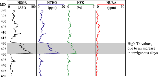
Mineralogy / Geochemistry The concentrations of the three main radioactive elements in the formation can often be used to give an indication of the mineralogy and/or geochemistry. For example, high Th values may be associated with the presence of heavy minerals, particularly in channel sand deposits overlying an erosional unconformity. Increased Th values may also be associated with an increased input of terrigenous clays (Hassan et al. 1976) (Figure 2).  
fig2

Figure 2. Spectral gamma tay data from Hole 1124C, showing high Th values in a mudstone unit between 420-430 mbsf.

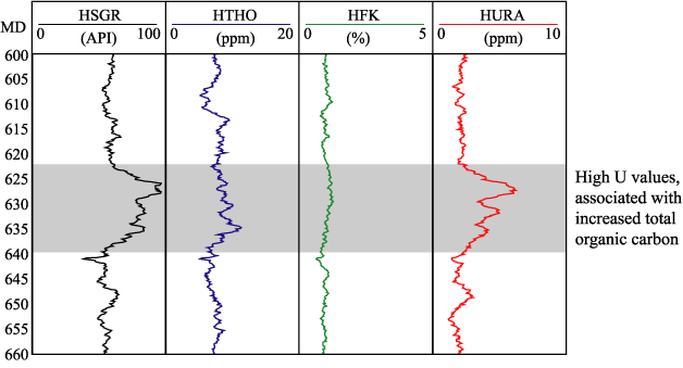
Increases in U are frequently associated with the presence of organic matter. For example, particularly high U concentrations (>~5 ppm) and low Th/U ratios (<~2) occur in black shale deposits (Adams & Weaver 1958). In the Ocean Drilling Program, a correlation can often be observed between the U log and the total organic carbon values measured in the core (Figure 3)
 
fig4

Figure 3. Spectral gamma-ray data from Hole 1172D, showing high U values in an organic-bearing claystone unit between ~662-640 mbsf.

 
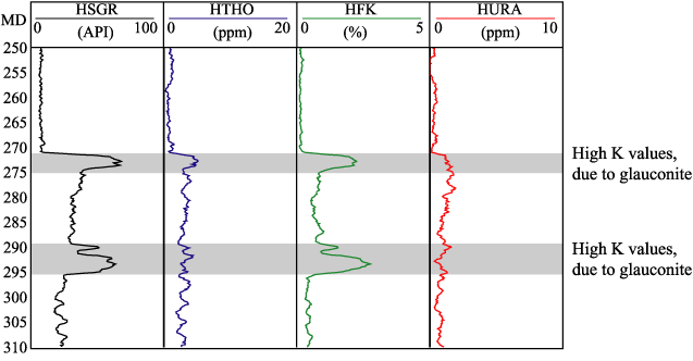
In sandstones, high K values may be caused by the presence of potassium feldspars or micas (Humphreys & Lott 1990, Hurst 1990). Glauconite usually produces a very distinctive, almost diagnostic spike in the K log (Figure 4).
   
fig3

Figure 4. Spectral gamma-ray data from Hole 1171D, showing high K values due to the presence of glauconite.

   
In ocean floor volcanics, K can become significantly enriched in secondary alteration minerals, which are typically found where the formation is more permeable and intense fluid-rock interactions can occur (Brewer et al. 1992). An example of this can be seen in ODP Hole 896A, where the lowest K values occur in relatively impermeable massive flows, whereas higher and more variable K concentrations can be correlated with the more permeable pillow lavas and breccias (Brewer et al, 1998).
More quantitative attempts have been made to derive a mineralogy from the spectral gamma-ray log, which generally involve cross-plotting Th against K (Quirein 1982), PEFL against K (Schlumberger 1991), or PEFL against Th/K (Schlumberger 1991). However, the validity of these methods is questionable (Hurst 1990), and it is unlikely that they are applicable in a wide variety of sedimentary environments.  
Cyclostratigraphic analysis
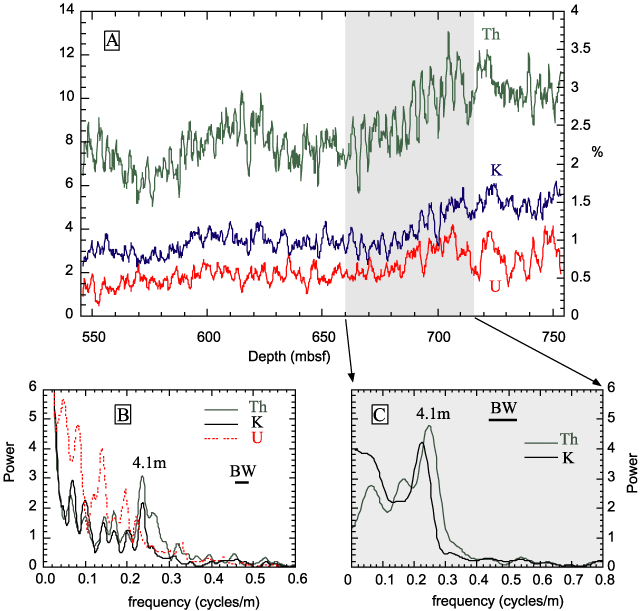
Spectral gamma-ray data can also be used for cyclostratigraphic analysis of the formation, to help identify the frequency of paleoceanographic and/or climatic change (Figure 5). Data acquired by the recently developed Lamont Multisensor Gamma ray Tool will be particularly valuable for time series analysis, due to its very high resolution (~8 cm).
 
fig5

Figure 5. Spectral gamma-ray data (A) and preliminary analysis (B and C) from 1170F. The power spectrum show the results of spectral analysis over the entire logged section (B) and the interval where the Th and K data show the most pronounced cyclicity (C)

 
References

Adams, J.A. & Weaver, C.E. 1958. Thorium-uranium ratios as indicators of sedimentary processes: example of concept of geochemical facies. Bulletin American Association of Petroleum Geologists 42(2), 387-430.

Brewer, T.S, Pelling, R., Lovell, M.A. & Harvey, P.K. 1992. The validity of whole rock geochemistry in the study of  ocean crust: a case study from ODP Hole 504B. In: Parson, L.M., Murton, B.J. & Browning, P. (eds), Ophiolites and their modern ocean analogues. Geological Society of London Special Publication No. 60, 263-278.

Brewer, T.S, Harvey, P.K., Lovell, M.A., Haggas, S., Williamson, G & Pezard, P. 1998. Ocean floor volcanism: constraints from the integration of core and downhole logging measurements. In : Harvey, P.K. & Lovell, M.A. (eds), Geological Society of London Special Publication No. 136, 341-362. 

Doveton, J.D. 1991. Lithofacies and geochemical facies profiles from nuclear wireline logs: new subsurface templates for sedimentary modelling. In: Franseen, E.K., Watney, W.L., Kendall, C.J. & Ross, W. (eds), Sedimentary modelling-computer simulations and methods for improved parameter definition. Kansas Geological Society Bulletin 233, 101-110.

Ellis, D.V., 1987. Well logging for earth scientists. Elsevier, Amsterdam.

Hassan, M., Hossin, A. & Combaz, A. 1976. Fundamentals of the differential gamma ray log interpretation technique. SPWLA 17th Annual. Symposium Transactions Paper 8, 1-7.

Heslop, A. 1974. Gamma-ray log response of shaly sandstones. Trans. SPWLA, McAllen, Texas.

Hurst, A. 1990. Natural gamma-ray spectrometry in hydrocarbon-bearing sandstones from the Norwegian Continental Shelf. In: Hurst, A., Lovell, M.A. & Morton, A.C. (eds), Geological Application of Wireline Logs, Geological Society of London Special Publication No. 48, 211-222.

Humphreys, B. & Lott, G.K. 1990. An investigation into nuclear log responses of North Sea Jurassic sandstones using mineralogical analysis. n: Hurst, A., Lovell, M.A. & Morton, A.C. (eds) Geological Application of Wireline Logs, Geological Society of London Special Publication No 48, 223-240.

Quirein, J., Gardner, J.S. & Watson, J.T. 1982. Combined natural gamma ray spectral/lithodensity measurements applied to complex lithologies. SPE 11143, 57th Annual Fall Technical Conference and Exhibition of SPE and AIME, New Orleans, Sept. 26-29.

Rider, M. 1990. Gamma-ray log shape used as a facies indicator: critical analysis of an oversimplified method. In: Hurst, A., Lovell, M.A. & Morton, A.C. (eds), Geological application of wireline logs. Geological Society of London Special Publication No 48, 27-37.

Rider, M. 1996. The Geological Interpretation of Well Logs: Caithness (Whittles Publishing). Schlumberger, 1991. Log interpretation charts. SMP-7006, Schlumberger Wireline & Testing. Serra, O. & Sulpice, L. 1975. Sedimentological analysis of shale-sand series from well logs. Transactions of the SPWLA 16th Annual Logging Symposium, paper W.  

Borehole Compensated Sonic Tool (BHC*)

Borehole Compensated Sonic Tool (BHC*)

Description
bhc The BHC sonde measured the time required for a compressional sound wave to travel through one foot of formation. The BHC consisted of an upper and lower transmitter arranged symmetrically on either side of two pair of receivers. The spacings T1-R2 and T1-R4 were 3 and 5 feet apart, as well as the spacings T2-R3 and T2-R1. The transmitters were pulsed alternately and the transit time of the compressional wave in the formation, measured in microseconds per foot, was given by: Δt=1/2 (T1R4-T1R2+T2R1-T2R3)
The BHC was used during the Deep Sea Drilling Project from 1975-1982 and the Ocean Drilling Program from 1987-1998. It was also deployed during IODP Expedition 302.


Applications

Porosity and “pseudo density”: The sonic transit time can be used to compute porosity by using the appropriate transform, and to estimate fracture porosity in carbonatic rocks. In addition, it can be used to compute a “pseudodensity” log over sections where this log has not been recorded or the response was not satisfactory.

Seismic impedance: The product of compressional velocity and density can be used to compute synthetic seismograms for time-depth ties of seismic reflectors.

Sonic waveform analysis: If a refracted shear arrival is present, its velocity can be computed from the full waveforms, and the frequency content and energy of both compressional and shear arrivals can also be determined.


Environmental Effects One common problem is cycle skipping: a low signal level, such as that occurring in large holes and soft formations, can cause the far detectors to trigger on the second or later arrivals, causing the recorded Δt to be too high. This problem can also be related to the presence of fractures.
Transit time stretching appears when the detection at the further detector occurs later because of a weak signal. Finally, noise peaks are caused by triggering of detectors by mechanically induced noise, which causes the Δt to be too low.


Log Presentation
Delay times (µsec/ft) were usually displayed along with gamma ray and resistivity data.


Tool Specifications
Temperature rating: 350° F (175° C)
Pressure rating: 20 psi (138 MPa
Diameter: 3.625 in (9.21 cm)


Main Outputs
DT: Delay time (5 ft) (µsec/ft)
TT1: Transit time 1 (5 ft) (µsec)
TT2: Transit time 2 (5 ft) (µsec)
TT3: Transit time 3 (5 ft) (µsec)
TT4:  Transit time 4 (5 ft) (µsec)


Deployment Notes
The BHC could be run alone or in combination with resistivity and gamma ray tools.


*®trademark of Schlumberger

3-Component Well Seismic Tool (WST-3*)

3-Component Well Seismic Tool (WST-3*)

Description
wst-3 The WST-3 was a Schlumberger three axis check shot tool for both check shot and vertical seismic profiles (VSP). It consisted of three geophones that pressed against the borehole wall and recorded the acoustic waves generated by an air gun located near the sea surface. The tool was designed specifically for use in an offset VSP experiment, where a remote seismic source would be fired from a second ship.
The WST-3 was used on several ODP legs in 2002 and 2003 and on IODP expedition 305.


Applications
VSP data acquired by the WST-3 are useful for:
  • Providing seismic interval velocities which can be compared to the rock sequence intersected by the borehole
  • Placing the borehole results in their proper setting with respect to the seismically defined structure of the oceanic crust and mantle
  • Correlating borehole lithology with the up-going seismic reflected wavefield
  •  Predicting structure and lithology changes below the drill hole
  • Estimating physical properties of rock on seismic scales by studying particle motion and downhole seismic attenuation. In check shot mode, the WST-3 data can be used to produce a depth-travel time tie and to calibrate the sonic logs and determine accurate drilling depths and their relative position with respect to targets on the seismic reflection profiles.


Tool Specifications
Mechanical:
Temperature rating: 350° F (175° C)
Pressure rating: 20 kpsi (138 MPa)
Diameter: 3.625 in (9.21 cm)
Length: 19.9 ft (6.07 m)
Weight: 310 lbs (141 kg)
Sampling interval: 1, 2 or 4 msec (selectable)
Minimum hole diameter: 5 in (12.7 cm) with “short” arms
Maximum hole diameter: 19 in (48.3 cm) with “long” arms
Maximum logging speed: Stationary
Sensors:
Axis: 3 axis
Geophone: 3 axis
Geophone type: SM4 (3ea gimbaled)
Geophone frequency: 10 Hz
Damping: 60 dB
Sensitivity per axis: 83 V/m/sec or 0.8 V/in/sec at 25° C
Low-cut frequency: 0.2 Hz
Low-cut slope: 18 dB per octave
High-cut frequency : 250 Hz for 1 msec or 125 Hz for 2 and 4 msec sampling
High-cut slope: 36 dB per octave
Digitization: Downhole
Sampling rate: 1, 2 or 4 msec (selectable)
ADC resolution: 11 bit + sign
Autoranger steps: Five 6 dB steps
Preamplifier gain: 40 – 160 dB by 6 dB steps for each axis
Dynamic range per waveform (shot): 90 dB
Total dynamic range: 156 dB
Input noise level: 2 μV
Anti-aliasing filters: 330 Hz / 24 dB per octave


Deployment Notes The WST-3 could be used in both checkshot and vertical seismic profile experiments. A remote seismic source was required for an offset survey, while a traditional check shot survey or zero-offset VSP could be completed with existing equipment on the JOIDES Resolution.
For each type of experiment, the deployment routine for the WST-3 was approximately the same. The main difference was simply the location of the source and the handling of the trigger pulse. For a check shot, a 120 in³ air gun was suspended by buoys at a depth of 3 mbsl, offset 48.5 m from the hole on the portside. The WST-3 was clamped against the borehole wall at intervals of approximately 50m, and the air gun fired five to seven times. The resulting waveforms were stacked and a travel time was determined from the median of the first breaks in each trace. These check shot experiments attempted to reproduce the seismic reflection profiling by simulating a similar geometry and source frequency.

The WST-3 was typically the last tool run and was always run alone. At each selected station, a seismic shot was produced at the sea surface using either air or water guns. Schlumberger provided a blast hydrophone for synchronizing the gun pulse with the system timer.

The WST-3 was sensitive to pipe noise and ringing of pipe following a shot. Efforts were made to reduce pipe noise at each station. If time and resources permitted, a drill string packer was deployed to dampen the banging motion of the pipe against the borehole. In addition, a 50 to 75 m distance was left between the tool and the bottom of pipe.


* ®trademark of Schlumberger

Schlumberger Wireline Tools

Schlumberger Wireline Logging Tools

Logging-While-Coring Resistivity-at-the-Bit* System

Logging-While-Coring Resistivity-at-the-Bit* System

Description
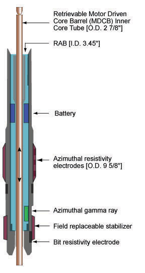
lwc_rab_coringThe Logging-While-Coring (LWC-RAB) system, developed jointly by USIO/LDEO, Schlumberger Drilling and Measurements, and USIO/TAMU, took advantage of existing logging, drilling and coring technologies and synthesized them into a powerful new exploration system.
Recent improvements in battery technology enabled the reformatting of the electronics in an 8-inch Schlumberger Resistivity-at-the-Bit (RAB) tool. By placing smaller batteries in the drill collar wall, an existing ODP core barrel can pass through the RAB to carry out coring operations while making simultaneous azimuthal geophysical measurements. The coring tool technology consists of the Motor Driven Core Barrel (MDCB) system developed by USIO/TAMU, which needed only minor modifications and the fabrication of crossovers and drilling subs.
The assembled system was tested at the Genesis test facility in Sugarland, Texas, and successfully deployed for the first time during ODP Leg 204.


Applications
• Core-log data integration capability
• Assessment of borehole breakout for local and regional stress analyses
• Detection of formation heterogeneity using azimuthal resistivity images
• Lithology characterization


Log Presentation
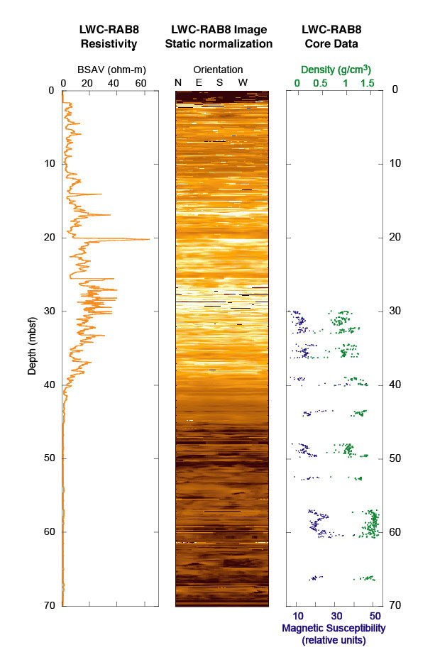
Resistivity image and average resistivity data from the LWC-RAB plotted with physical properties data from cores.
lwc_RAB


Tool Specifications
Temperature rating: 300° F (149° C)
Pressure rating: 18 kpsi (124 MPa)
Length: 13 ft (4 m)
Weight: 2,400 lbs (1,090 kg)
API nominal collar outside diameter: 8.25 in (21 cm)
Maximum outside diameter: 9 to 12.25 in (23 to 31 cm)
Minimum bit size: 9.75 in (25 cm)
Maximum bit size: 12.25 in (31 cm)
Flow range: 0-1,200 gpm
Maximum curvature – sliding: 13 deg/100 ft (13 deg/31 m)
Maximum rotary torque: 23,000 ft-lbf (7,010 m-lbf)
Minimum operating RPM: 30 rpm
Uphole connection: 6-5/8 Reg box
Downhole connection: 6-5/8 Reg box


Measurement Specifications 
Gamma Ray
Range: 0-250 GAPI
Accuracy: 7%
Vertical resolution: 6 in (15.24 cm)
Azimuthal resistivity
Range: 0.2-20,000 Ω.m
Accuracy: 5% (0.2-200 Ω.m); 20% (200-2,000 Ω.m) n/a (>2,000 Ω.m)
Vertical resolution: 2-3 in (5.08-7.62 cm)
Ring resistivity
Range: 0.2-20,000 Ω.m
Accuracy: 5% (0.2-2,000 Ω.m); 20% (>2,000 Ω.m)
Vertical resolution: 2-3 in (5.08-7.62 cm)
Bit resistivity 
Range: 0.2-20,000 Ω.m
Accuracy: 5% (0.2-2,000 Ω.m); 20% (>2,000 Ω.m)
Vertical resolution: 12-24 in (30.5-61 cm)

*®trademark of Schlumberger

Schlumberger LWD Tools

Schlumberger LWD Tools